


-
Traditionally, in quantum mechanics, when one solves the Schrodinger equations, Dirac equations, or Klein-Gordon equations, to obtain the bound states of an atom, at some points, the sign of a parameter’s square root has to be chosen, and the choice leads either to “usual” solution or “anomalous” solution[1].
The traditionally discarded “anomalous” solutions can be explained as quantum states occupied by electrons under the “usual” Bohr ground level. The bounding energy is comparable to the rest mass of the electron, and therefore is called to be deep Dirac level (DDL), electron deep level, or relativistically bounded level in literatures[2-3].
The existence of the DDLs are debated theoretically, as well as experimentally. Some experimental phenomenons have been explained as existence of the DDLs[4–6], but being questioned by others[7–10].
With the development of high intensity lasers, nowadays, the electrons, and even the nuclei, can be accelerated by the lasers to relativistic energies in a very short distance like 1 µm, and therefore may populate atoms to the DDL states. Due to the very short distance from the electron’s DDL orbit to the nuclei, the electron capture (EC) life time can be changed greatly. Therefore one can use the EC rate as an indicator of the DDL state. In this paper, We propose a novel nuclear indicator of DDL existing, for the first time. The nuclear capture life time will be dramatically changed if DDL is formed. We will also discuss the possibilities of using high intensity laser facilities to test the existence of the hypothetical DDLs.
-
For simplicity, here we only briefly give the DDL solution of the Klein-Gordon equation. The DDL solutions of other equations like the relativistic Schrodinger equation and Dirac equation can be found in Ref. [11]. Considering the Klein-Gordon equation of a hydrogen-like atom[3],
$$ \left[ \left( {\rm{i}}\hbar\partial_t -U \right)^2 +\hbar^2 c^2 \Delta \right] \psi_t = m_0^2 c^4 \psi_t, $$ (1) where
$ \hbar $ is the Plank constant,$ c $ is the speed of light,$ m_0 $ is the mass of electron,$ U(r) = -\frac{Z \alpha\hbar c}{r} $ is the coulomb potential,$ \alpha $ is the fine structure constant,$ r $ is distance between electron and nuclei, and$ Z $ is the charge of the nuclear. This equation has solution of Ref. [3],$$ \psi_t = \frac{r_0^{s-3/2} r^{-s} {\rm e}^{-r/r_0}}{2^{s-1/2}\sqrt{\pi \varGamma(3-2s)}} {\rm{e}}^{-{\rm{i}} E_0 t/\hbar}, $$ (2) where
$ \varGamma(x) $ is the gamma function,$ t $ is time. The corresponding energy$ E_0 $ and the orbit$ r_0 $ are:$$ E_0 = m_0 c^2\frac{Z\alpha}{\sqrt{s}}, $$ (3) and
$$ r_0 = \frac{\hbar}{m_0c}\frac{1}{\sqrt{s}}. $$ (4) The
$ s = \frac{1}{2}(1-\sqrt{1-4Z^2\alpha^2})\simeq 0 $ solution is the normal non-relativistic one, the Bohr state. In this case, the corresponding energy, orbit, and the wave function are:$$ E_0 = m_0 c^2\left(1-\frac{1}{2}Z^2\alpha^2 + ...\right)\simeq m_0 c^2-Z^2\times13.6\; {\rm{eV}}, $$ (5) $$ r_0\simeq\frac{\hbar}{m_0c}\frac{1}{Z \alpha}\simeq \frac{0.53}{Z}\; \mathop {\rm{A}}\limits^ \circ , $$ (6) $$ \psi_0\simeq\frac{ e^{-r/r_0}}{r_0^{3/2}\sqrt{\pi}} {\rm{e}}^{-{\rm{i}} E_0 t/\hbar}. $$ (7) The
$ s = \frac{1}{2}(1+\sqrt{1-4Z^2\alpha^2})\simeq 1 $ solution is is the “anomalous” one, i.e. the so-called DDL level. In this case, the energy, orbit, and wave function can be simplified as,$$ E_0^\# = m_0 c^2\cdot Z\alpha\simeq m_0 c^2-(511-3.72\cdot Z)\; {\rm{keV}}, $$ (8) $$ r_0^\#\simeq\frac{\hbar}{m_0c}\simeq 0.003\,9\, \mathop {\rm{A}}\limits^ \circ , $$ (9) $$ \psi_0^\#\simeq\frac{ r^{-1}{\rm e}^{-r/r_0^{\#}}}{\sqrt{2\pi r_0^{\#}}} {\rm{e}}^{-{\rm{i}} E_0^\# t/\hbar}. $$ (10) As one can see, taking
$ Z = 1 $ as an example, in the case of the DDL, the electron is deeply bounded to 0.507 3 MeV, compared with the well-known Bohr case 13.6 eV. The DDL's orbit is only about 390 fm away from the nucleus, compared with the Bohr orbit, 0.53$ \mathop {\rm{A}}\limits^ \circ $ .Because the wave function
$ \lim\limits_{r \to 0}\psi_0^{\#} = \infty $ , this “un-physical” solution was rejected in textbooks like Ref. [1]. However, the infinity comes from the assumption that the nucleus is point-like, and therefore the Coulomb potential is infinite at$ r = 0 $ . Even though, the system's wave function$ \psi_0^{\#} $ and momentum$ p_0^{\#} = -{\rm{i}}\hbar\,\partial_r\psi_0^{\#} $ are still square integrable. In fact, the wave function Eq. (2) has already been normalized in$ r\in[0, \infty) $ . -
As shown above, if DDL exists, a free electron can drop to a DDL, and X-ray with energy of about 0.5 MeV will be emitted. Because we do not observe so many energetic photons in our normal environment, that means directly populating DDLs via photon-emission must be highly forbidden.
First, the DDLs may be populated via electron-positron pair effect. When a relativistic electron approaches a nucleus,
$ e^-e^+ $ pairs can be produced through the following two processes[12-13]:$$ Z+e^- \rightarrow Z+ 2 e^- +e^+, $$ (11) and
$$ Z+e^- \rightarrow Z+e^-+ \gamma\rightarrow Z+ 2 e^- +e^+, $$ (12) where the
$ Z $ represents nuclear with charge$ z $ . The previous process can create electron-positron pair directly in the nuclear coulomb field. The later process has two steps, i.e., in the first step, generating a$ \gamma $ photon with energy larger than$ >2m_e c^2 $ , and then the gamma decays to an electron-positron pair. In both cases, the electron could be captured to the DDL. The larger the electrical field, i.e. the closer to the nuclear, the higher the possibility is. Therefore, the electrons produced near the nuclei have higher chance to be bounded to be DDLs. Because the electron in the DDL is much closer to the nucleus, it has higher possibility to be caught which results in a short EC life time. The life time of the nuclei's electron capture decay may serve as an indicator of DDLs.Secondly, the DDL may also be produced by mechanism called Nuclear Excitation by Electron Transition (NEET)[14]. When an electron moves from an outside orbit to an inner one, the energy difference
$ \Delta E_e $ between the two orbits is usually carried away by X rays or Auger electrons. However, it is possible that this energy$ \Delta E_e $ can also excite the atomic nucleus. The NEET has been founded in several nuclei, e.g., 197Au, 189Os, and 193Ir etc.[15-16]. With the high intensity lasers, the DDL may be produced through the NEET mechanism.With the development of high intensity laser technologies, the intensities of today's laser could be as high as
$ 10^{22} $ W/cm2[17]. With high intensity laser, the electron-positron pairs have been experimentally observed[18]. When an$ e^-e^+ $ pair is created near nuclei, the positron escapes due to the coulomb field, and the electrons may be caught to the DDLs. Due to the electron quiver effect, electrons in high-intensity laser fields can acquire relativistic energy, and then the NEET may be triggered.For the DDL purposes, the high-intensity lasers have relatively clean background. In a typical high-intensity laser experiment, a laser pulse's duration is normally shorter than nanosecond. The radiation produced in this time interval include X-rays,
$ \gamma $ -rays, neutrons, high energy electrons, positrons, high energy ions, and radioactive isotopes. The photons (X-ray and$ \gamma $ -ray) decline immediately in nanoseconds. After the original pulse, the high energy electrons, as well as the ions, fly away from the target, and hit on materials around to have Bremsstrahlung$ \gamma $ -ray or other neutrons. This process may last another several nanoseconds. The positrons may last longer, but their annihilation energy is smaller than$ 2m_0c^2 = 1.022 $ MeV if the detectors capture one photon from the annihilation, and equals to 1.022 MeV if capture both.However, from the experimental point of view, the positrons themselves only are hardly to be used as an indicator of the DDLs. After all, a lot of positrons, as well as different energy photos, are produced by lasers in a time interval smaller than one nanosecond. It's very hard to trace the history of a positron experimental in this circumstance.
There are two kinds of
$ \gamma $ background in the typical high-intensity laser experiment: laser induced and ambient gamma. The later one comes from cosmic rays or the radiation of the ambient materials. The laser background after roughly about 100 ns almost disappears. The ambient$ \gamma $ background normally is very small compared with the laser$ \gamma $ background at$ t \simeq 0 $ , but as the measurement time goes longer and longer, it will dominate. Therefore, a window of about 100 ns to 1 min is reasonable for the DDL detecting.After about 100 ns, almost all observed photons with
$ E_\gamma>1.1 $ MeV must come from 5 sources: neutron capture reactions, activated radioactive isotopes, ambient sources, the energy fluctuation of e+ annihilation which is a gaussian distribution with the center at 1.022 MeV, and the possible EC from DDLs. The first two sources have their own characteristic$ \gamma $ -ray, and can be distinguished from the DDL cases. The ambient background can be compressed by choosing a proper time window, let's say, from$ 10^2 $ to$ 10^{11} $ ns. The positron background can be compressed by choosing a proper energy window. Base on the discussion above, the laser-induced EC decay may be an ideal probe for the DDL studies. -
Let’s consider the EC process,
$$ ^A_Z X+e^- \rightarrow\, ^{\,\ \ A}_{Z-1}Y+\nu_e. $$ (13) The EC decay probability per time unit is given by Fermiis golden rule,
$$ \lambda = \frac{{2\pi }}{\hbar }|\left\langle {f\left| {\hat O} \right|i} \right\rangle {|^2}{\rho _f}, $$ (14) where
$ i $ ,$ f $ are initial and final states respectively,$ \rho_f $ is the neutrino final states per energy unit, and$ \hat{O} $ is the weak interaction operator.In the initial state, there are one proton, one electron, and other nucleons in
$ ^A_Z X $ ,$ \left| i \right\rangle = \left| {p,e} \right\rangle \left| {_{Z - 1}^{A - 1}Y} \right\rangle $ . In the finial state, there have one neutron, one neutrino, and other nucleons in$ ^{\,\,\,\,\,\,A}_{Z-1}Y $ ,$ \left| f \right\rangle = \left| {n,\nu } \right\rangle \left| {_{Z - 1}^{A - 1}Y} \right\rangle $ . Since the operator$ \hat{O} $ acts only on weak interaction participants, the EC decay rate is roughly proportional to the possibility of finding the electron in the nuclear volume[19],$$ \lambda\propto \int_0^{r_n} |\psi_e |^2\cdot 4\pi r^2 {\rm{d}}{{r}}, $$ (15) where
$ \psi_{\rm e} $ is the electron's wave function, and$ r_{\rm n} $ is radius of the nucleus. Here we use the assumption that the nucleon's wave function is constant in the nuclear volume. Furthermore, the coulomb interaction difference between the normal Bohr state and the DDL is very small compared with the strong interaction inside the nuclei. Therefore, the other parts of the matrix for the Bohr level and the DDL are roughly same. Defining$ T_{1/2} $ to be the half life of capturing an electron from normal Bohr level, and$ T_{1/2}^{\#} $ from DDL, their ratio can be simplified as[19-20]:$$ \frac{T_{1/2}^{\#}}{T_{1/2}^{}} \simeq\left[ \frac{Q^{}}{Q^{\#}} \frac{|\psi_0^{}(r_{\rm n})|}{|\psi_0^{\#}(r_{\rm n})|} \right]^2 $$ (16) $$ \simeq \left[ (\frac{1}{1-m_0 c^2/Q}) \frac{|\psi_0^{}(r_{\rm n})|}{|\psi_0^{\#}(r_{\rm n})|} \right]^2, $$ (17) where the
$ Q^{} $ and$ Q^{\#} $ is the reaction Q-value for Bohr and the DDL states respectively. The$ \frac{|\psi_0^{}(r_{\rm n})|}{|\psi_0^{\#}(r_{\rm n})|} $ is the ratio of the electron wave functions evaluated at the nuclear surface$ r = r_{\rm n} $ . And also take$ Q^{\#} = Q-m_0c^2 $ .From Eq. (7) and (10), we have
$$ \frac{|\psi_0^{}(r_{\rm n})|}{|\psi_0^{\#}(r_{\rm n})|} = \frac{\sqrt{2}(r_0^{\#})^{1/2}r_{\rm n}}{r_0^{3/2}}\exp[{r_{\rm n}/r_0^{\#}-r_{\rm n}/r_0}]. $$ (18) Since
$ r_{\rm n} $ is in order of fm level,$ r_0^\# $ is about 390 fm, and$ r_0 $ is about 0.53$ \mathop {\rm{A}}\limits^ \circ $ , we have$ \exp[{r_{\rm n}/r_0^{\#}-r_{\rm n}/r_0}]\simeq 1 $ . The equation can be re-written as,$$ \frac{|\psi_0^{}(r_n)|}{|\psi_0^{\#}(r_n)|} \simeq \frac{r_n}{r_0} \sqrt{2Z\alpha}, $$ (19) insert it to the Eq. (17), we have
$$ \frac{T_{1/2}^{\#}}{T_{1/2}^{}} \simeq \frac{2Z\alpha}{(1-m_0 c^2/Q^{})^2} \left(\frac{r_{\rm n}}{r_0}\right)^2. $$ (20) The results, chosen as examples, are shown as
$ T_{1/2}^{\rm{(DDL1)}} $ in Table 1.Table 1. The new life time of several radioactive nuclei if the DDL exist.
$ T_{1/2}^{(0)} $ represents the original half life of the corresponding nucleus.Nucleus $ Q $/MeV Z $ T_{1/2}^{(0)} $ $ T_{1/2}^{\rm{(DDL1)}} $ $ T_{1/2}^{\rm{(DDL2)}} $ 7Be 0.861 4 53.2 d 21 ms 52 ms 11C 1.982 6 20.3 m 18 μs 19 μs 13N 2.220 7 10.0 m 14 μs 16 μs 15O 2.757 8 122 s 4.3 μs 4.8 μs 23Mg 4.056 12 11.3 s 1.5 μs 1.9 μs 30P 4.232 15 2.50 m 47 μs 64 μs 53Fe 3.742 26 8.51 m 1.3 ms 2.9 ms 62Cu 3.958 29 9.67 m 2.2 ms 5.9 ms 63Zn 3.367 30 38.47 m 10 ms 30 ms 64Cu 1.675 29 12.7 h 0.28 s 0.7 s We also numerically solve the Eq. (1) with a more realistic potential, specifically, assuming that the charge is evenly distributed in the nucleus. The potential U in Eq. (1) has the form:
$$ U(r) = \left\{ {\begin{array}{*{20}{l}} { - \dfrac{{Z\alpha \hbar c}}{r}}&{}&{r > {r_{\rm n}}},\\ { - \dfrac{{Z\alpha \hbar c{\mkern 1mu} {r^2}}}{{r_{\rm n}^3}}}&{}&{r\leqslant{r_{\rm n}}}. \end{array}} \right. $$ (21) Once obtaining the numerical wave functions, the EC decay ratio were then calculated according to Eq. (15). The results are shown as
$ T_{1/2}^{\rm{(DDL2)}} $ in Table 1. As an example, the numerically-solved wave functions for 62Cu's Bohr state and DDL are shown in Fig. 1.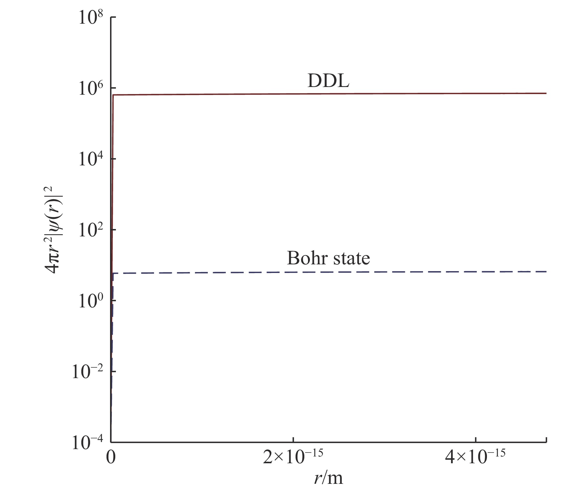
Figure 1. A comparison of the numerical evaluation of
$4\pi r^2|\psi(r)|^2 (r < r_{\rm n})$ for the 62Cu's Bohr state (dash line) and DDL (solid line).The present studies reveal that the nuclei listed in the Table 1 are possible candidates for the laser DDL studies. They will be prepared at accelerators or nuclear reactors in advance, and then server as laser targets. They can be obtained by one-nucleon transferring reactions and relatively easier to be prepared. Furthermore, because theirs
$ T_{1/2}^{\rm{(DDL)}} $ are much longer than 100 ns, but relatively shorter regarding the cosmic and ambient radiation backgrounds (look the argument in Sec. 3), a high signal-to-noise ratio can be achieved if using these nuclei. -
In this work we provide a new experimental method to explore the deep Dirac levels. The DDLs may be populated by high intensity lasers through the mechanism of
$ e^+e^- $ pair or the NEET. Because the DDL orbit is very close to the nucleus, the electron capture (EC) rate can be enhanced greatly. We estimate that the EC rate will be over$ 10^7 $ times higher if the DDL exist. The characteristic EC decay$ \gamma $ -ray could be used as the indicator of the DDL's existence. We suggest a detecting time window, from 100 ns to 1 min, which can avoid both the laser-induced$ \gamma $ -ray at$ t = 0 $ and the ambient$ \gamma $ -ray. We also provide several candidate nuclei which can be relatively easily created in laser setups. Their relatively high decay energies can benefit the detecting signal-to-noise ratios. We expect that this new laser-induced EC decay method will help to understand more about the long-existing DDL puzzle.
-
摘要: 多年以来,很多不同的理论预言了深度狄拉克态(DDL)的存在。然而,DDL的存在依然存在很大的争议,急需进行验证。随着超强激光技术的提高,可以利用超强激光把电子加速到相对论能量,也可以产生正负电子对,引发核反应等。强激光所提供的这种极端环境也为探索DDL带来新可能。本文提出一个新的探测DDL的方法,即以原子核的轨道电子俘获寿命在强激光等离子体中的变化为探针,探测DDL是否存在。计算表明,若DDL存在,轨道电子俘获寿命变化可达7个量级,从而有望在现有超强激光条件下探测DDL。Abstract: Various theories have predicted the deep Dirac levels (DDLs) in atoms for many years. However, the existence of the DDL is still under debating, and need to be confirmed. With the development of high intensity lasers, nowadays, electrons can be accelerated to relativistic energies by high intensity lasers. Furthermore, electron-positron pairs can be created, and nuclear reactions can be ignited, which provide a new tool to explore the DDL related fields. In this paper, we propose a new experimental method to study the DDL levels by monitoring nuclei's orbital electron capture life time in plasma induced by high intensity lasers. The present study reveal that if a DDL exists, a nuclear electron capture rate could be enhanced by factor of over
$ 10^7$ , which makes it a very sensitive method for the DDL detecting. -
Figure 1. A comparison of the numerical evaluation of
$4\pi r^2|\psi(r)|^2 (r < r_{\rm n})$ for the 62Cu's Bohr state (dash line) and DDL (solid line).Table 1. The new life time of several radioactive nuclei if the DDL exist.
$ T_{1/2}^{(0)} $ represents the original half life of the corresponding nucleus.Nucleus $ Q $ /MeVZ $ T_{1/2}^{(0)} $ $ T_{1/2}^{\rm{(DDL1)}} $ $ T_{1/2}^{\rm{(DDL2)}} $ 7Be 0.861 4 53.2 d 21 ms 52 ms 11C 1.982 6 20.3 m 18 μs 19 μs 13N 2.220 7 10.0 m 14 μs 16 μs 15O 2.757 8 122 s 4.3 μs 4.8 μs 23Mg 4.056 12 11.3 s 1.5 μs 1.9 μs 30P 4.232 15 2.50 m 47 μs 64 μs 53Fe 3.742 26 8.51 m 1.3 ms 2.9 ms 62Cu 3.958 29 9.67 m 2.2 ms 5.9 ms 63Zn 3.367 30 38.47 m 10 ms 30 ms 64Cu 1.675 29 12.7 h 0.28 s 0.7 s  下载: 导出CSV
-
[1] SCHIFF L I. Quantum Mechanics[M]. 3rd ed. New York: McGraw-Hill Publishing Company, 1968. [2] DOMBEY N. Phys Lett A, 2006, 360: 62. doi: 10.1016/j.physleta.2006.07.069 [3] NAUDTS J. arXiv: physics/0507193 (2005). [4] PHILLIPS J, MILLS R L, CHEN X. J App Phys, 2004, 96: 3095. doi: 10.1063/1.1778212 [5] MILLS R, RAY P. J Phys D, 2003, 36: 1535. doi: 10.1088/0022-3727/36/13/316 [6] VA'VRA J. arXiv: 1304.0833 (2013). [7] JOVIĆEVIĆ S, SAKAN N, IVKOVIĆ M, et al. J App Phys, 2009, 105: 013306. doi: 10.1063/1.3046587 [8] RATHKE A. New J Phys, 2005, 7: 127. doi: 10.1088/1367-2630/7/1/127 [9] PHELPS A V. J App Phys, 2005, 98: 066108. doi: 10.1063/1.2010616 [10] DE CASTRO A S. Phys Let A, 2007, 369: 380. doi: 10.1016/j.physleta.2007.05.006 [11] PAILLET J L, MEULENBERG A. J Cond Mat Nucl Sci, 2016, 18: 50. [12] KUCHIEV M Y, ROBINSON D. Phys Rev A, 2007, 76: 012107. doi: 10.1103/PhysRevA.76.012107 [13] MILSTEIN A I, MÜLLER C, HATSAGORTSYAN K Z, et al. Phys Rev A, 2006, 73: 062106. doi: 10.1103/PhysRevA.73.062106 [14] DZYUBLIK A Y. Phys Rev C, 2013, 88: 054616. doi: 10.1103/PhysRevC.88.054616 [15] KISHIMOTO S, YODA Y, SETO M, et al. Phys Rev Lett, 2000, 85: 1831. doi: 10.1103/PhysRevLett.85.1831 [16] AHMAD I, DUNFORD R W, ESBENSEN H, et al. Phys Rev C, 2000, 61: 051304. doi: 10.1103/PhysRevC.61.051304 [17] DI PIAZZA A, MÜLLER C, HATSAGORTSYAN K, et al. Reviews of Modern Physics, 2012, 84: 1177. doi: 10.1103/RevModPhys.84.1177 [18] NERUSH E N, KOSTYUKOV I Y, FEDOTOV A M, et al. Phys Rev Lett, 2011, 106: 035001. doi: 10.1103/PhysRevLett.106.035001 [19] BAMBYNEK W, BEHRENS H, CHEN M, et al. Rev Mod Phys, 1977, 49: 77. doi: 10.1103/RevModPhys.49.77 [20] BAHCALL J N. Phys Rev, 1963, 132: 362. doi: 10.1103/PhysRev.132.362 -

 点击查看大图

图(1) / 表 (1)
计量
- 文章访问数: 529
- HTML全文浏览量: 146
- PDF下载量: 33
- 被引次数: 0


 甘公网安备 62010202000723号