


-
The fact that the
$ \tau $ is the only lepton heavy enough to decay into hadrons makes the hadronic$ \tau $ lepton decays a priceless test of the strong interaction at low energy in the light flavor sector.$ \tau $ lepton decay is important to learn about weak interaction as well as strong interaction[1]. Therefore, it is important and meaningful to explore theoretically the$ \tau $ lepton decay, especially it is closely connected with the recent proposed large research facility of the Super Tau-Charm Facility of China (STCF). However, currently the theoretical investigation is scarce on$ \tau $ physics.In this paper I will present a novel algebraic method proposed recently to investigate the
$ \tau $ lepton decays and also present some interesting applications.$ \tau $ decays into$ \nu_{\tau} $ and a pair of mesons make up for a sizeable fraction of the$ \tau $ decay width in PDG[2] in which several modes are well measured for$ \tau^-\! \to \!\nu_{\tau} {\rm{PP}} $ and$ \tau^-\! \to\! \nu_{\tau} {\rm{PV}} $ , here$ {\rm{P}} $ denotes the pseudoscalar meson and$ {\rm{V}} $ the vector meson. However, very surprisingly, there are no$ \tau^- \!\to\! \nu_{\tau} {\rm{VV}} $ reported. Actually, the pseudoscalar and vector mesons differ only by the spin arrangement of the quarks, hence it should be possible to relate the rates of decay for two pseudoscalar mesons and the related pseudoscalar-vector or vector modes, for instance,$ \tau^- \!\to\! \nu_{\tau} K^{0} K^{-}, $ $\nu_{\tau} K^{0} K^{*-}, \;\nu_{\tau} K^{*0} K^{-}, \;\nu_{\tau} K^{*0} K^{*-} $ .Now we present a novel approach and obtain the analytical amplitudes for
$ \tau $ decays with no any free parameter. The formalism is obtained in the standard model (SM)[3], leading to a different interpretation of the role played by$ G $ -parity in these decays. We evaluate and also predict the invariant mass distributions and branching ratios of rates for the different$ \tau $ reactions.Then we discuss some interesting applications in
$ \tau $ decays, including the polarization amplitudes and tests on the nature of scalar resonances or axial-vector resonances. We extend the analytical amplitudes on$ \tau $ decay to models Beyond the Standard Model (BSM) with$ (\gamma^\mu- \alpha \gamma^\mu \gamma_5) $ structure[4] ($ \alpha = 1 $ for the SM). It is the first time to investigate polarization amplitudes in$ \tau $ decays. We find some observables are very sensitive to the value of$ \alpha $ , which should stimulate experimental work to investigate possible physics BSM. The$ f_0(980) $ and$ a_0(980) $ are predicted as dynamically generated resonances from the interaction of pseudoscalar mesons in coupled channels[5] and have been successfully tested in many reactions[6]. Now we firstly open up a new direction in the$ \tau $ decays to test the nature of scalar resonances[7]. In the chiral unitary approach that the$ f_1(1285) $ ,$ b_1(1235) $ ,$ h_1(1170) $ ,$ h_1(1380) $ ,$ a_1(1260) $ and two poles of the$ K_1(1270) $ are dynamically generated axial-vector resonances from the interaction of vector-pseudoscalar meson in coupled channels[8], these resonances also have been successfully tested in many reactions[6]. Now we also firstly open up a new direction in the$ \tau $ decays to test the nature of axial-vector resonances[9]. We predict the invariant mass distributions and branching ratios of rates, finding these numbers are within measurable range. -
The first step is to look at the
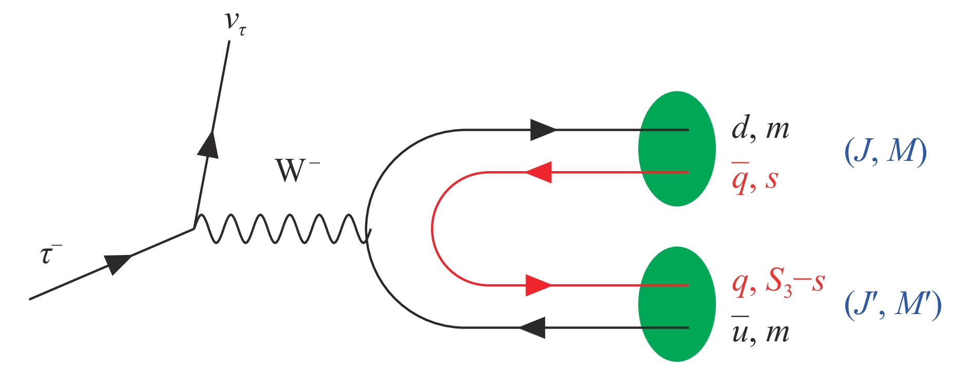
$ \tau^- \to \nu_{\tau} q \bar{q} $ decay for the Cabibbo-favored$ d\bar{u} $ production. We can obtain the Cabibbo-suppressed mode substituting the$ d $ quark by an$ s $ quark. However, we are interested in the production of two mesons, not just one, as it would come from the mechanism when$ q \bar{q} $ merge into a meson. The procedure to produce two mesons is hadronization by creating a new$ q \bar{q} $ pair with the quantum numbers of the vacuum. This is depicted in Fig. 1.
Figure 1. (color online)Hadronization of the primary
$d\bar{u}$ pair to produce two mesons,$s$ is the third component of the spin of$\bar{q}$ propagating as a particle, while$S_3-s$ is the third component of the spin of$q$ , where$S_3$ is the third component of the total spin$S$ of$\bar{q}q$ .Where
$ J M (J' M') $ are the final angular momenta and third component of the two mesons produced. The sum over the$ M' $ and$ M $ components was done[3] and also keep track of the individual$ M' $ and$ M $ contributions[4].The matrix element of the Hamiltonian of the weak interaction in SM is given by
$$ H = {\cal{C}} L^\alpha Q_\alpha \,, $$ (1) where the
$ {\cal{C}} $ contains the couplings of the weak interaction, playing no role since we are only concerned about ratios of rates. The leptonic current is given by$$ L^\mu = \big\langle \bar u_\nu |\gamma^\mu- \gamma^\mu\gamma_5| u_\tau\big\rangle, $$ (2) and the quark current
$$ Q^\mu = \big\langle \bar u_d|\gamma^\mu-\gamma^\mu\gamma_5|v_{\bar u}\big\rangle. $$ (3) For the spinors at rest
$ \bar{u}\gamma^0 u \to \langle \chi^{\prime}| 1 |\chi \rangle $ , and$ \bar{u}\gamma^i \gamma_5 u \to \langle \chi^{\prime} | \sigma_i |\chi \rangle $ , here$ \sigma_i $ is the Pauli matrices and$ \chi $ is spin wave function with bispinors. Then the matrix elements$$ \begin{array}{l} Q_0 = \big\langle \chi^{\prime} | 1 | \chi \big\rangle \equiv M_0 \, , \quad Q_i = \big\langle \chi^{\prime} | \sigma_i |\chi \big\rangle \equiv N_i \, , \end{array}$$ (4) and one can find more details about the derivation of matrix elements
$ M_0 $ and$ N_i $ terms[3]. -
The first interesting application is about the polarization amplitudes to
$ \tau $ leptonic decays[4]. In this work we extend the formalism to a case, with the operator$ \gamma^\mu -\alpha\gamma^\mu \gamma_5 $ , that can account for different models BSM. We study the$ \tau^- \!\to\! \nu_{\tau} K^{*0} K^{-} $ reaction for the different polarizations of the$ K^{*0} $ [4].The final transition amplitudes for the
$J \!=\! 1,\; J'\! =\! 0$ (vector- pseudoscalar) are obtained by1)
$M \!= 0 \!$ $$ \begin{split} \overline{\sum} \sum \left|t\right|^2 =& \frac{1}{m_\tau m_\nu} \frac{1}{6}\left(\frac{1}{4 \pi}\right)^2 \,\Big\{ \left(E_\tau E_\nu + p^2 \right) + \, \\ & 2 \alpha^2 \left(E_\tau E_\nu - p^2 \right) \Big\}\, , \end{split} $$ (5) 2) for
$\!M = 1 \!$ $$ \begin{split} \overline{\sum} \sum \left|t\right|^2 =& \frac{1}{m_\tau m_\nu} \frac{1}{6}\left(\frac{1}{4 \pi}\right)^2 \,\Big\{(E_\tau E_\nu + p^2) + \, \\ & 2 \alpha (E_\nu\! +\!E_\tau) p \!+\! \big[2E_\tau E_\nu \!+\!(E_\nu \!-\!E_\tau) p \big] \alpha^2 \Big\} \, , \end{split} $$ (6) 3) for
$ M = -1 $ $$ \begin{split} \overline{\sum} \sum \left|t\right|^2 =& \frac{1}{m_\tau m_\nu} \frac{1}{6}\left(\frac{1}{4 \pi}\right)^2 \,\Big\{(E_\tau E_\nu + p^2)- \, \\& 2 \alpha (E_\nu \!+\!E_\tau) p \!+\! \big[2E_\tau E_\nu \!-\!(E_\nu \!-\!E_\tau) p \big] \alpha^2 \Big\} \, , \end{split}$$ (7) where
$ p $ is the momentum of the$ \tau $ in the$ M_1 M_2 $ (with$ M1, M2 $ pseudoscalar or vector mesons) rest frame given by$$ \begin{split} & p = \frac{\lambda^{1/2}\big(m^2_\tau,m^2_\nu,M_{\rm{inv}}^{2 (M_1 M_2)}\big)}{2 M_{\rm{inv}}^{(M_1 M_2)}} \, , \\ & E_\tau = \sqrt{m_\tau^2+p^2}, \quad E_\nu = p \,, \end{split} $$ (8) with
$ \lambda(x,y,z) = x^2+y^2+z^2-2xy-2xz-2yz $ .Finally the differential width is given
$$ \frac{ {\rm{d}}\varGamma}{{\rm{d}} M_{\rm{inv}}^{(K^{*0} K^-)}} = \frac{2\,m_\tau 2\, m_\nu}{(2\pi)^3} \frac{1}{4 m^2_\tau}\, p_\nu {\widetilde p_1}\, \overline{\sum} \sum \left|t\right|^2 \,, $$ (9) where
$ p_\nu $ is the neutrino momentum in the$ \tau $ rest frame and$ {\widetilde p_1} $ the momentum of$ K^{*0} $ in the$ K^{*0}K^- $ rest frame.The total differential width is
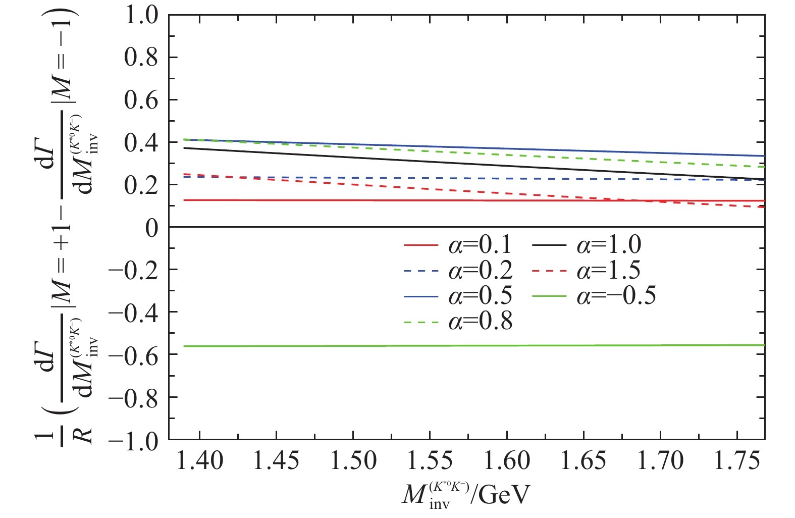
$$ \begin{split} R = & \frac{{\rm{d}} \varGamma}{{\rm{d}} M_{\rm{inv}}^{(K^{*0} K^-)}}\Big|_{M = +1} + \frac{{\rm{d}} \varGamma}{{\rm{d}} M_{\rm{inv}}^{(K^{*0} K^-)}}\Big|_{M = 0} + \, \\ & \frac{{\rm{d}} \varGamma}{{\rm{d}} M_{\rm{inv}}^{(K^{*0} K^-)}}\Big|_{M = -1} \, . \end{split}$$ (10) We find that the polarization amplitudes vary very much with different values of
$ \alpha $ . In particular we find a magnitude$\frac{1}{R} \big[\frac{{\rm{d}} \varGamma}{{\rm{d}} M_{\rm{inv}}^{(K^{*0} K^-)}}\big|_{M = +1}- \frac{{\rm{d}} \varGamma}{{\rm{d}} M_{\rm{inv}}^{(K^{*0} K^-)}}\big|_{M = -1} \big]$ , which is extremely sensitive to$ \alpha $ . The results are shown in Fig. 2, it is shown that this magnitude is very sensitive to the$ \alpha $ parameter and even changes sign for some value of$ \alpha $ . It is obviously to be most suited to investigate possible physics BSM.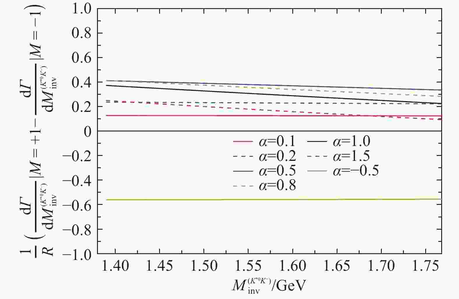
Figure 2. (color online)The difference as a function of
$ \alpha.$ -
Now firstly we open up a new direction to test the nature of scalar resonances
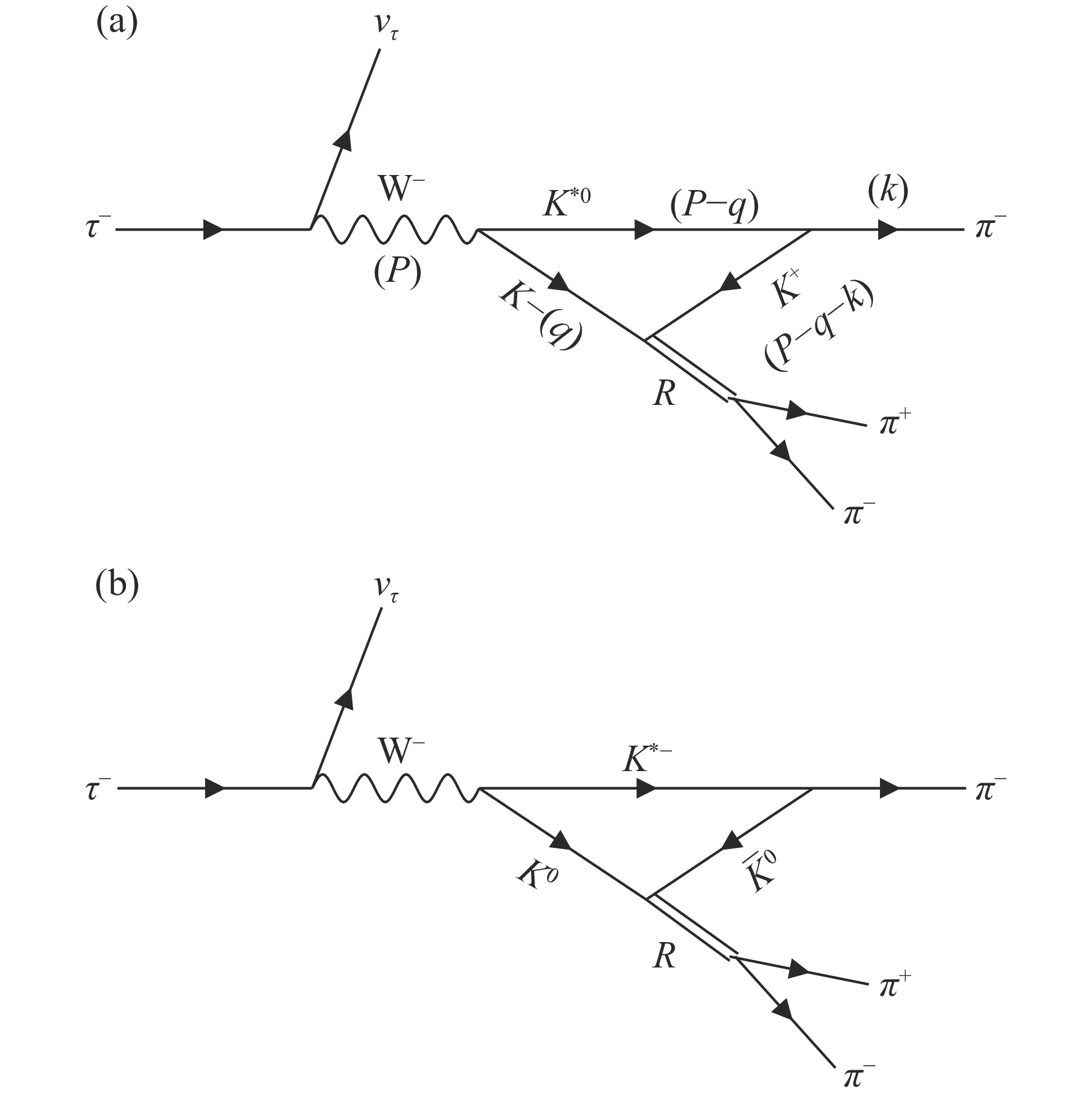
$ f_0(980) $ and$ a_0(980) $ in the$ \tau $ decays. In the present work the$ \tau^- \to \nu_\tau \pi^- f_0(980) $ and$ \tau^- \to \nu_\tau \pi^- a_0(980) $ reactions are investigated[7].In Fig. 3 we show the triangle mechanism to produce the
$ f_0(980) $ state via$ \tau \to \nu_\tau K^{*0} K^- $ ($ K^0 K^{*-} $ ) followed by$ \bar{K}^{*} \to \pi^- K $ and the posterior fusion of$ K\bar{K} $ . Similarly, the process producing the$ a_0(980) $ state is depicted in Fig. 4.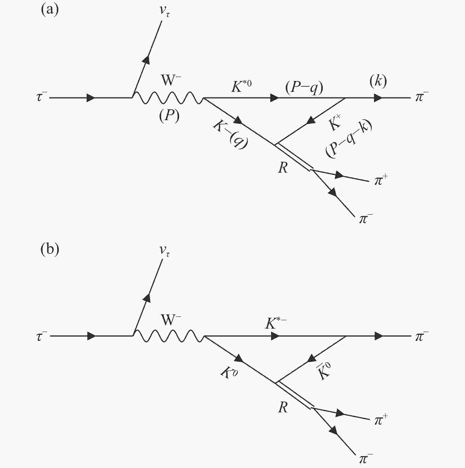
Figure 3. Diagram for the decay of
$\tau^- \to \nu_\tau \pi^- \pi^+ \pi^- $ . The double line, labeled R, indicating the$K\bar K\to\pi^+\pi^-$ scattering amplitudes. The brackets in figure (a) indicate the momenta of the particles.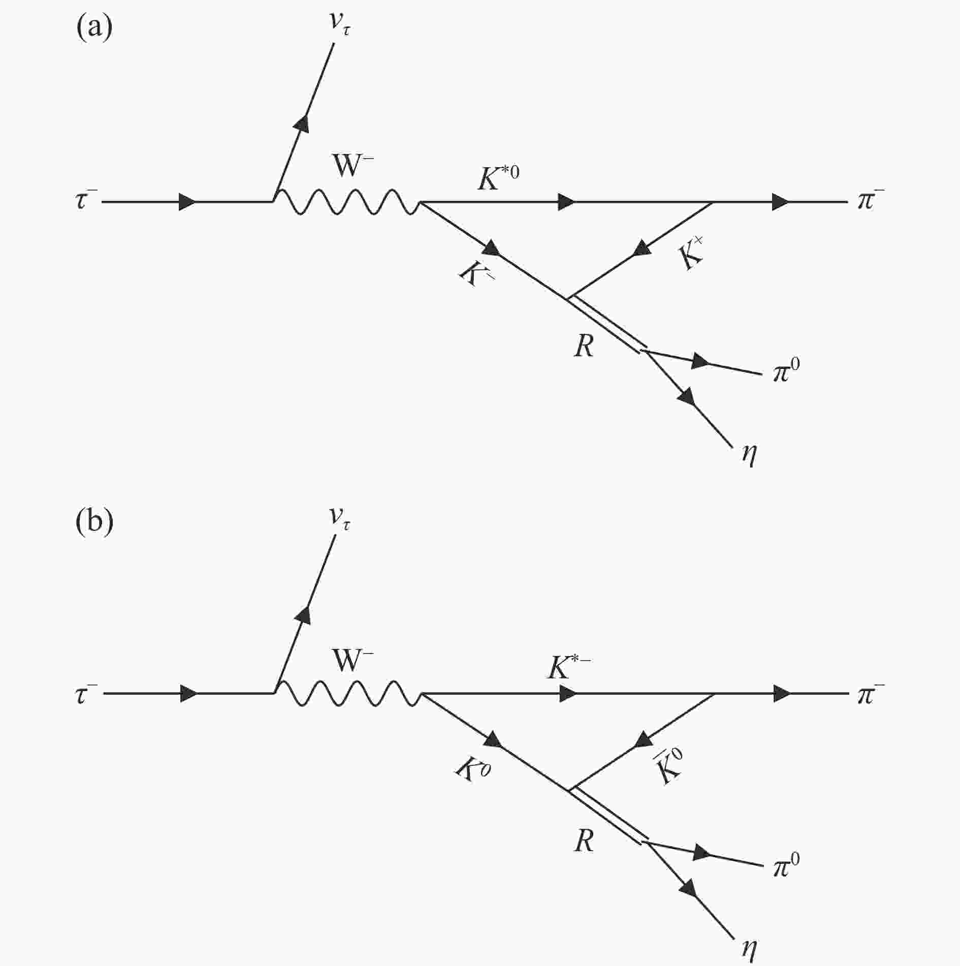
Figure 4. Diagram for the decay of
$\tau^- \to \nu_\tau \pi^- \pi^0 \eta $ .We obtain that the
$ M_0 $ terms cancel for the production of$ f_0(980) $ and add for the production of$ a_0(980) $ . This is, the$ f_0(980) $ production proceeds via the$ N_i $ term and the$ a_0(980) $ production via the$ M_0 $ term. Since$ \pi^- f_0(980) $ has negative$ G $ -parity and$ \pi^- a_0(980) $ positive$ G $ -parity, we confirm that the$ M_0 $ term in the loop corresponds to positive$ G $ -parity and the$ N_i $ term to negative$ G $ -parity[3].For the production of
$ \pi^- f_0(980) $ $$ \begin{split} \overline{\sum} \sum \big|t\big|^2 =& \frac{{\cal{C}}^2}{m_\tau m_\nu} \left(E_\tau E_\nu -\frac{1}{3} p^2 \right) \frac{1}{3} \frac{1}{(4 \pi)^2} \times \\ & k^2 \, \big|t_L\big|^2 \, g^2\, \big|\,2 \,t_{K^+ K^-,\pi^+ \pi^-}\big|^2 \,.\; \; \end{split} $$ (11) Similarly, for the production of
$ \pi^- a_0(980) $ $$ \begin{split} \overline{\sum} \sum \big|t\big|^2 =& \frac{{\cal{C}}^2}{m_\tau m_\nu} \left(E_\tau E_\nu + p^2 \right) \frac{1}{6} \frac{1}{(4 \pi)^2} \times \\ & k^2 \big|t_L\big|^2 \, g^2\, \big|\,2 \,t_{K^+ K^-,\pi^0 \eta}\big|^2 \, .\; \; \; \end{split} $$ (12) For
$ \tau^- \to \nu_\tau \pi^- \pi^+ \pi^- $ decay, the double differential mass distribution for$ M_{\rm{inv}}(\pi^+ \pi^-) $ and$ M_{\rm{inv}}(\pi^- f_0) $ is given by$$ \begin{split} &\frac{1}{\varGamma_{\tau}}\frac{{\rm{d}}^2 \varGamma}{{\rm{d}} M_{\rm{inv}}(\pi^- f_0) {\rm{d}} M_{\rm{inv}}(\pi^+ \pi^-)} = \\ & \frac{1}{(2 \pi)^5} \frac{1}{\varGamma_{\tau}} k \, p'_{\nu}\, \widetilde{q}_{\pi^+} \, \frac{2 m_\tau 2 m_\nu}{4 M^2_\tau} \overline{\sum} \sum \left|t\right|^2 \, , \end{split}$$ (13) with
$$ \begin{split} & k = \frac{\lambda^{1/2}\big[M^2_{\rm{inv}}(\pi^- f_0), m_{\pi}^2, M^2_{\rm{inv}}(\pi^+ \pi^-)\big]}{2 M_{\rm{inv}}(\pi^- f_0)} \, , \\ & p'_{\nu} = \frac{\lambda^{1/2} \big[m_{\tau}^2,m^2_\nu, M^2_{\rm{inv}}(\pi^- f_0)\big]}{2 m_{\tau} } \, , \\ & \widetilde{q}_{\pi^+} = \;\;\frac{\lambda^{1/2} \big[ M^2_{\rm{inv}}(\pi^+ \pi^-),m^2_{\pi},m^2_{\pi}\big]}{2 M_{\rm{inv}}(\pi^+ \pi^-)}. \end{split}$$ (14) Similarly, for the
$ \tau^- \to \nu_\tau \pi^- \pi^0 \eta $ decay, we can get the double differential mass distribution for$ M_{\rm{inv}}(\pi^0 \eta) $ and$ M_{\rm{inv}}(\pi^- a_0) $ .In the calculation, the factor
$ \frac{{\cal{C}}^2}{\varGamma_{\tau}} = (2.10\pm0.40)\times 10^{-5}\,{\rm{MeV}}^{-3} $ is obtained by the experimental branching ratio of$ {\cal{B}} (\tau \to \nu_\tau K^{*0} K^-) $ decay and thus we can provide absolute values for the mass distributions.The loop function in Fig. 3 (a) is given by
$$ \begin{split} t_L =& \int \frac{{\rm{d}}^3 q}{(2 \pi)^3} \frac{1}{8 \omega_{K^{*}} \omega_{K^+} \omega_{K^-}} \frac{1}{k^0-\omega_{K^+}-\omega_{K^{*}}+i\dfrac{\varGamma_{K^{*}}}{2}} \, \left(2+ \frac{{{{q}}} \cdot {{k}}}{|{k}|^2}\right) \times \, \\[-1mm] &\frac{1}{P^0+\omega_{K^-}+\omega_{K^+}-k^0} \, \frac{1}{P^0 - \omega_{K^-} -\omega_{K^+}-k^0+ i \epsilon} \, \theta(q_{\rm{max}}-q^*)\times \, \\[1mm]& \frac{2P^0 \omega_{K^-} + 2 k^0 \omega_{K^+} -2(\omega_{K^-}+\omega_{K^+})(\omega_{K^-}+\omega_{K^+}+\omega_{K^{*}})}{P^0- \omega_{K^{*}}-\omega_{K^-}+i\dfrac{\varGamma_{K^{*}}}{2}} \,,\; \; \; \end{split} $$ (15) with
$ P^0 = M_{\rm{inv}}(\pi^- f_0) $ ,$ \omega_{K^-} = \sqrt{{{q}}^2+m_K^2} $ ,$ \omega_{K^+} = \sqrt{({{{q}}}+{{k}})^2+m_{K}^2} $ , and$ \omega_{K^*} = \sqrt{{{q}}^2+m_{K^\ast}^2} $ ,$$ \begin{split} k^0 =& \frac{M^2_{\rm{inv}}(\pi^- f_0)+m_{\pi}^2-M^2_{\rm{inv}}(\pi^+ \pi^-)}{2 M_{\rm{inv}}(\pi^- f_0)} \,, \\[1mm] k =& \frac{\lambda^{1/2}\big[M^2_{\rm{inv}}(\pi^- f_0), m_{\pi}^2, M^2_{\rm{inv}}(\pi^+ \pi^-)\big]}{2 M_{\rm{inv}}(\pi^- f_0)} \,, \\[1mm] {{{q}}}^* =& \bigg\{\Big[\frac{E_R}{M_{\rm{inv}}(\pi^- \pi^+)}-1\Big] \frac{{{{q}}} \cdot {{k}}}{|{k}|^2}+ \frac{q^0}{M_{\rm{inv}}(\pi^- \pi^+)} \bigg\} {{k}} + {{{q}}} \,. \; \; \; \; \end{split} $$ (16) Similarly, we can get the triangle amplitude for the
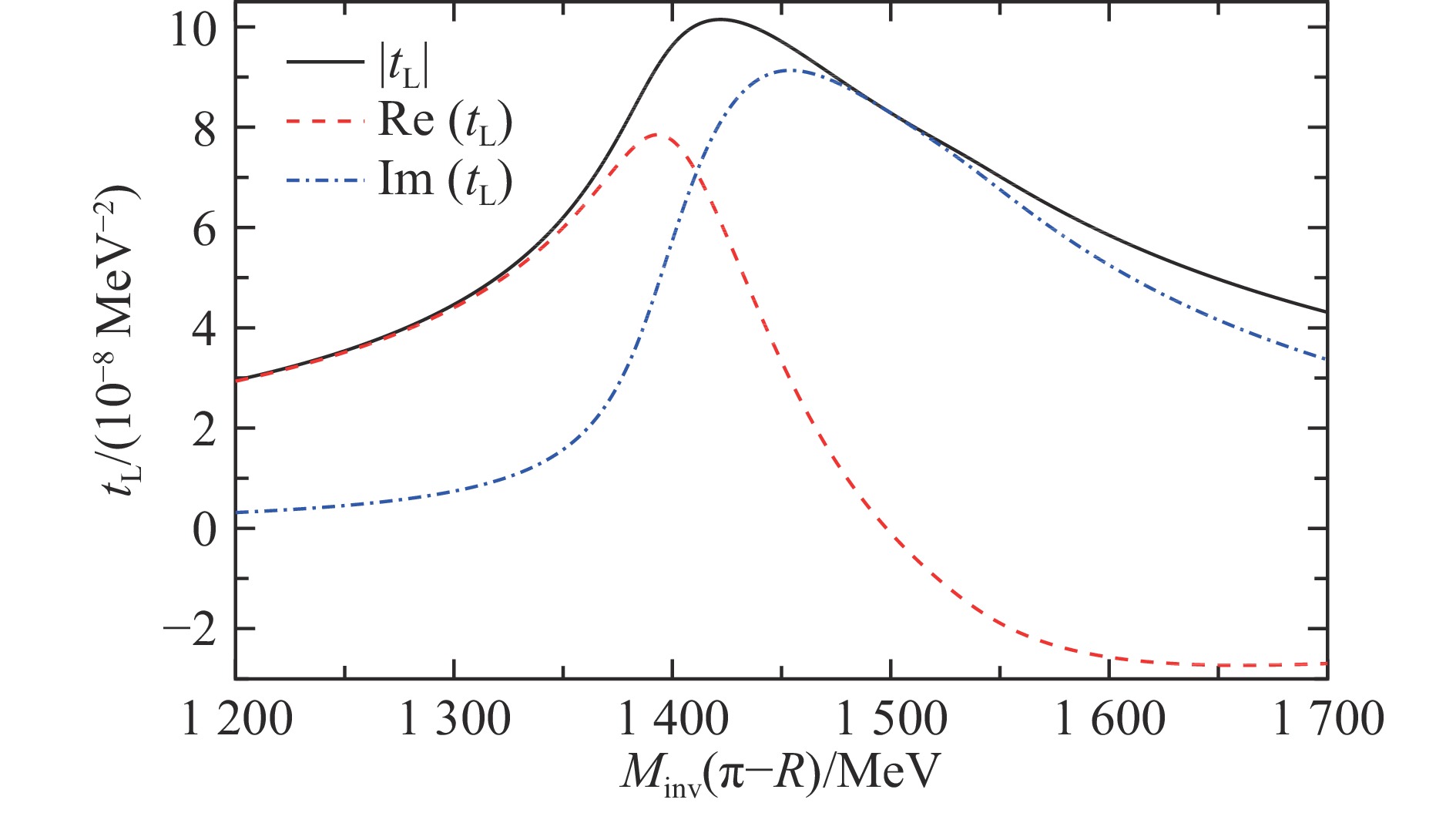
$ \pi^- a_0 $ case. Note that an$ i \epsilon $ in the propagators involving$ \omega_{K^{*}} $ is replaced by$ i\frac{\varGamma_{K^{*}}}{2} $ .In Fig. 5 we show the contribution of the triangle loop, the real, imaginary and the absolute value parts of
$ t_L $ as a function of$ M_{\rm{inv}}(\pi^- R) $ , with$ M_{\rm{inv}}(R) $ fixed at 985 MeV ($ R $ standing for$ f_0(980) $ or$ a_0(980) $ ). It can be observed that$ {\rm{Re}}(t_T) $ has a peak around 1 393 MeV, and$ {\rm{Im}}(t_T) $ has a peak around 1 454 MeV, and there is a peak for$ |t_T| $ around 1 425 MeV. The peak of the real part is related to the$ K^* K $ threshold and the one of the imaginary part, that dominates for the larger$ \pi^- R $ invariant masses, to the triangle singularity. This triangle mechanism has the same origin as the explanations for the COMPASS peak in$ \pi f_0(980) $ that was initially presented as the new resonance “$ a_1(1420) $ ”[10].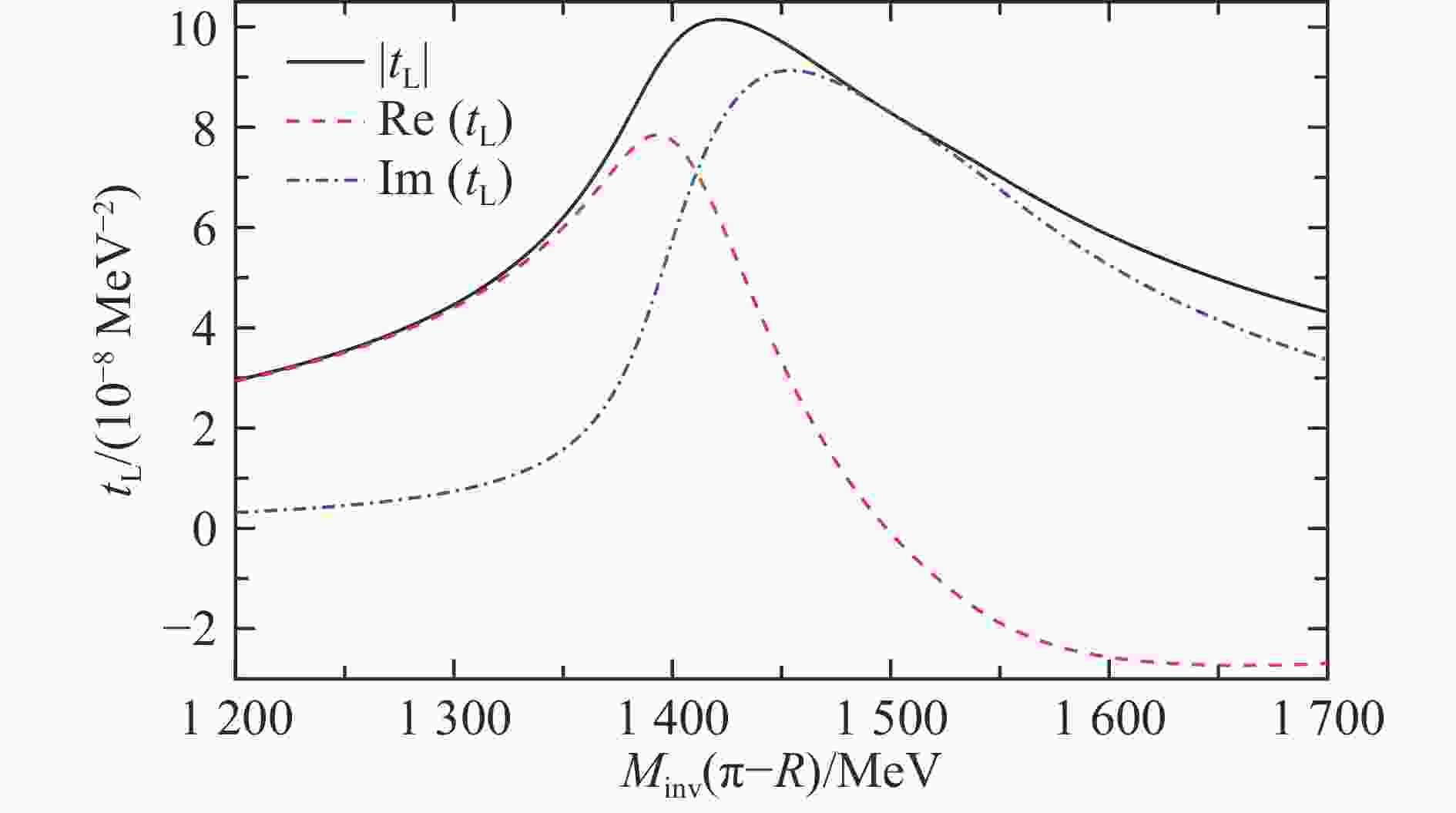
Figure 5. (color online)Triangle amplitude
${\rm{Re}} (t^{}_L)$ ,${\rm{Im}}(t^{}_L)$ and$|t^{}_L|$ , taking$M_{\rm{inv}}(R)$ = 985 MeV.In order to give a branching ratio for what an experimentalist would brand as
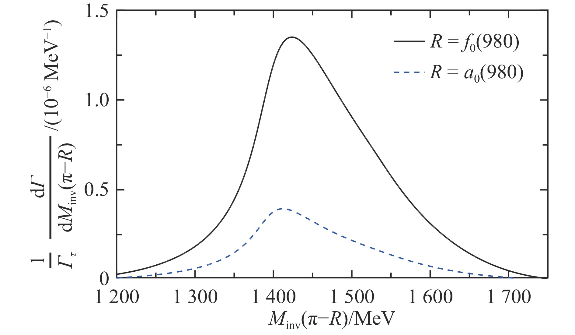
$ \pi^- f_0(980) $ or$ \pi^- a_0(980) $ decay, we integrate the strength of the double differential width and obtain$\frac{1}{\varGamma_{\tau}}\frac{{\rm d} \varGamma}{{\rm d} M_{\rm{inv}}(\pi^- R)}$ which is shown in Fig. 6. We see a clear peak of the distribution around$ 1\,423 $ MeV for$ \pi^- f_0 (980) $ production and$ 1\,412 $ MeV for$ \pi^- a_0 (980) $ production.
Figure 6. The mass distribution for
$\tau^- \to \nu_\tau \pi^- R$ .Integrating
$ \frac{{\rm{d}} \varGamma}{{\rm{d}} M_{\rm{inv}}(\pi^- R)} $ over$ M_{\rm{inv}}(\pi^- R) $ , we obtain the branching fractions$$ \begin{split} &{\cal{B}} (\tau^- \to \nu_\tau \pi^- f_0(980); \; \; f_0(980) \rightarrow \pi^+ \pi^-) \,= \\ & (3.9 \pm 0.8) \times 10^{-4} \,, \\ &{\cal{B}} (\tau^- \to \nu_\tau \pi^- a_0(980); \; \; a_0(980) \rightarrow \pi^0 \eta) \,=\\ & (7.1 \pm 1.4) \times 10^{-5} \,.\; \; \end{split} $$ (17) These numbers are within measurable range, since branching ratios of
$ 10^{-5} $ are quoted in the PDG. -
Now in the
$ \tau $ decays we firstly test the nature of axial-vector resonances. The decays of$ \tau \to \nu_\tau \pi A $ reactions, with$ A $ an axial-vector resonance, are investigated[9].The process proceeds through a triangle mechanism where a vector meson pair is first produced from the weak current and then one of the vectors produces two pseudoscalars, one of which reinteracts with the other vector to produce the axial resonance. The
$ G $ -parity is important to explicitly filter different states, and finally we obtain analytic formulas as follow:a)
$ G $ -parity positive axial states:$$ \begin{split} \overline{\sum} \sum \left|t\right|^2 =& \frac{{\cal{C}}^2}{m_\tau m_\nu} \,\frac{1}{(4\pi)^2} \, \frac{7}{6} \, \left(E_\tau E_\nu -\frac{1}{3} {p}^2 \right)\times \, \\ & g^2 \, k^2 \, \big|g_{A, K^* \bar{K}}\big|^2 \, \big|t_L(K^* \bar{K}^* )\big|^2 \, , \end{split} $$ (18) b)
$ G $ -parity negative axial states:$$ \begin{split} \overline{\sum} \sum \left|t\right|^2 =& \frac{{\cal{C}}^2}{m_\tau m_\nu} \,\frac{1}{(4\pi)^2} \, \frac{1}{3} \, (E_\tau E_\nu + {p}^2) \, g^2 \, k^2 \,\times \, \\ & \big|g_{A, K^* \bar{K}} t_L(K^* \bar{K}^*) + 2 \, D g_{A, \rho \pi} t_L(\rho\rho )\big|^2 \, , \; \; \; \end{split} $$ (19) The differential mass distribution for
$ M_{\rm{inv}}(\pi^- A) $ is given by$$ \begin{split} &\frac{1}{\varGamma_{\tau}} \frac{{\rm{d}} \varGamma}{{\rm{d}} M_{\rm{inv}}(\pi^- A)} = \\& \frac{1}{\varGamma_{\tau}} \, \frac{1}{(2 \pi)^3} \, \frac{2 m_\tau 2 m_\nu}{4 m^2_\tau} p_{\nu}\, \widetilde{p}_{\pi} \overline{\sum} \sum \left|t\right|^2 \, , \end{split} $$ (20) with
$$ \begin{split} & p_{\nu} = \frac{\lambda^{1/2} \big[m_{\tau}^2,m^2_\nu, M^2_{\rm{inv}}(\pi^- A)\big]}{2 m_{\tau} } \,, \\ &\widetilde{p}_{\pi} = \frac{\lambda^{1/2} \big[ M^2_{\rm{inv}}(\pi^- A),m^2_{\pi},m^2_{A}\big]}{2 M_{\rm{inv}}(\pi^- A)} \,. \end{split}$$ (21) and
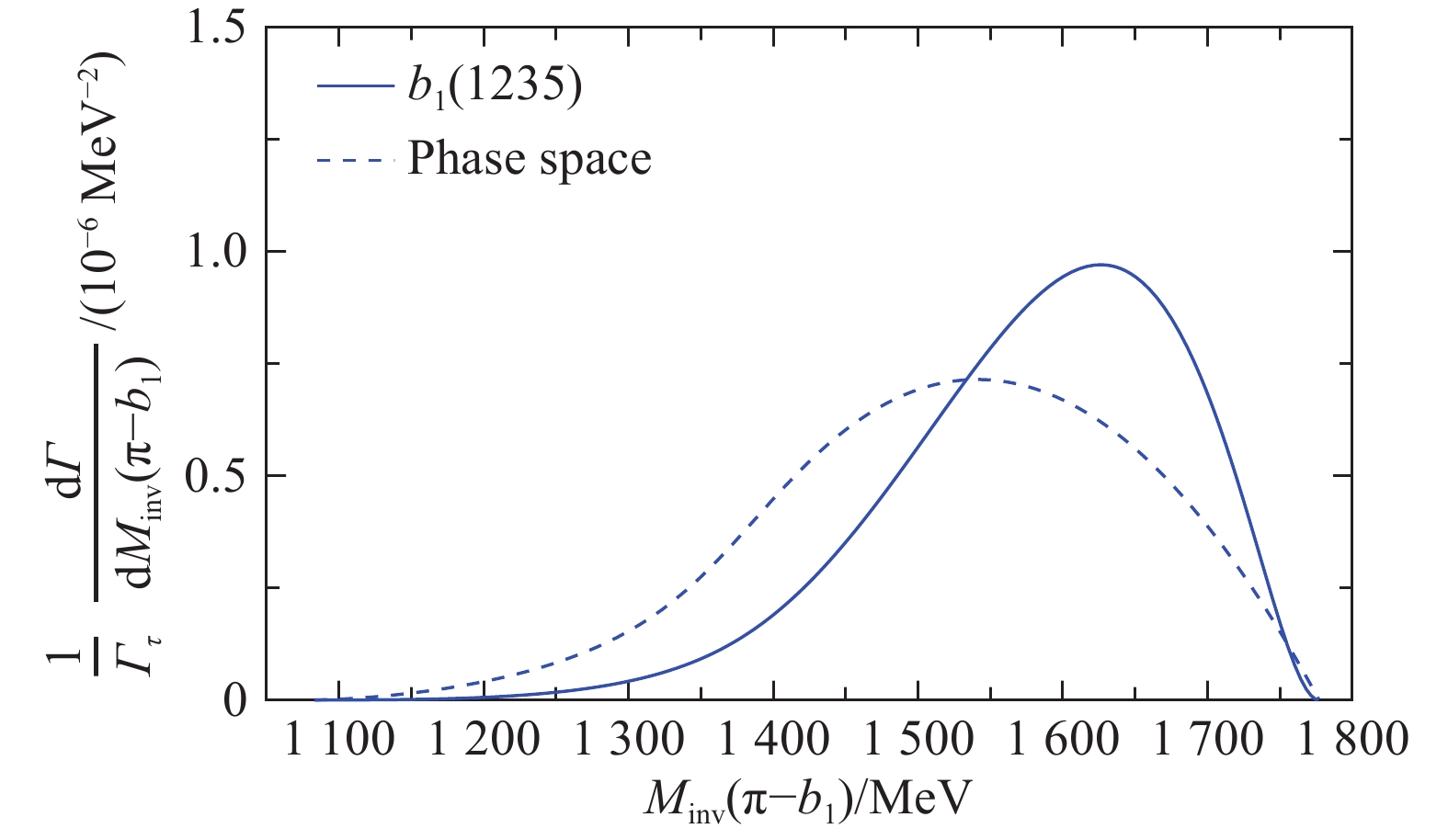
$ p $ is the momentum of the$ \tau $ in the$ \pi^- A $ rest frame.We make predictions for invariant mass distributions. In Fig. 7 we show the mass distribution for
$ \tau^- \to \nu_\tau \pi^- b_1(1235) $ decay, with$ G $ -parity positive$ b_1(1235) $ state.
Figure 7. (color online)Mass distribution for
$\tau^- \to \nu_\tau \pi^- b_1 (1235)$ decay.In Fig. 8 we also show the mass distribution for
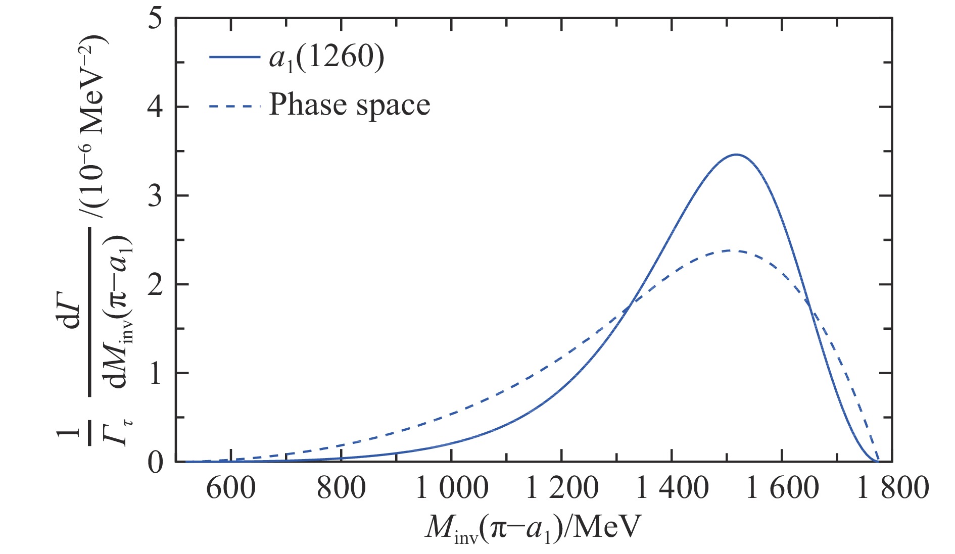
$ \tau^- \to \nu_\tau \pi^- a_1(1260) $ decay, with$ G $ -parity negative$ a_1(1260) $ state.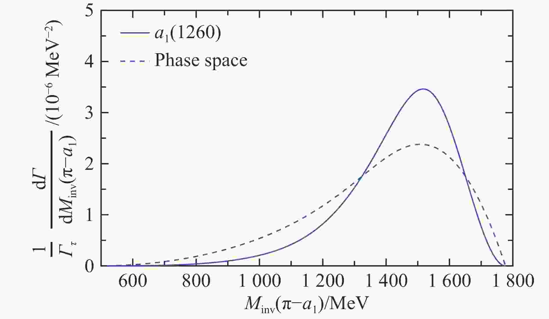
Figure 8. (color online)Mass distribution for
$\tau^- \to \nu_\tau \pi^- a_1 (1260)$ decay.We also give the decay of
$ \tau \to \nu_\tau K K_1(1270) $ . The axial-vector resonance$ K_1(1270) $ corresponds two states, one of them at$ 1195 $ MeV coupling mostly to$ K^* \pi $ , and another one at$ 1284 $ MeV coupling mostly to$ \rho K $ . Proceeding analogously to the previous cases, we obtain:a)
$ K_{1} (1) $ state:$$ \begin{split} \overline{\sum} \sum \left|t\right|^2 =& \frac{{\cal{C}}^2}{m_\tau m_\nu} \frac{1}{(4\pi)^2} \, g^2 \, k^2 \, |t_L(K^* \bar{K}^* )|^2 \, |g_{K_1, K^*\pi}|^2\times \, \\& \frac{1}{6} \left[\frac{1}{3}\left(E_\tau E_\nu + {p}^2 \right) + \frac{7}{6} \left(E_\tau E_\nu -\frac{1}{3} {p}^2 \right) \right] \, , \end{split} $$ (22) b)
$ K_{1} (2) $ state:$$\begin{split} \overline{\sum} \sum \left|t\right|^2 = & \frac{{\cal{C}}^2}{m_\tau m_\nu} \frac{1}{(4\pi)^2} \, g^2 \, k^2 \, |t_L(\rho\rho )|^2 \, (\sqrt{2})^2 \times \, \\ & \frac{1}{3}\left(E_\tau E_\nu + {p}^2 \right) \, \frac{4}{3} \, |g_{K_1, \rho K}|^2 \, , \end{split} $$ (23) Then in Figs. 9 and 10 and we get the differential mass distributions for
$ M_{\rm{inv}}(K^- K_1(1270)) $ and$ M_{\rm{inv}}(K^- K_2(1270)) $ cases, respectively,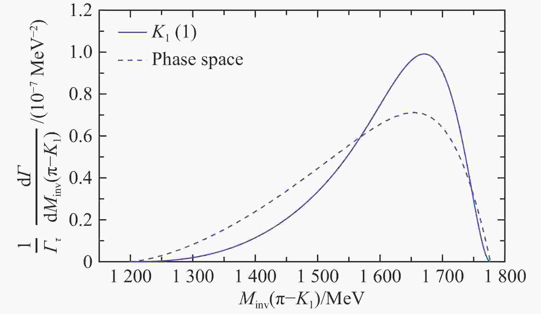
Figure 9. (color online)Mass distribution for
$\tau^- \to \nu_\tau K^- K_1(1) $ decay.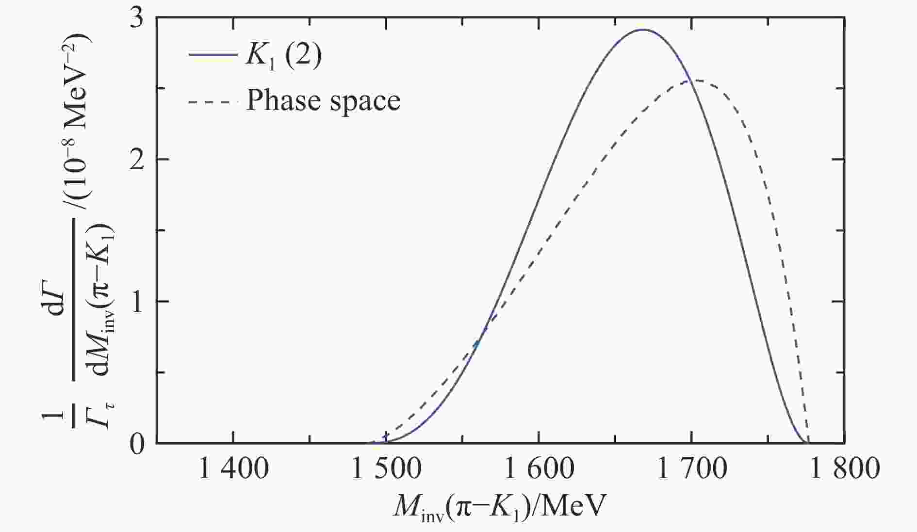
Figure 10. (color online)Mass distribution for
$\tau^- \to \nu_\tau K^- K_1(2) $ decay.From the experimental branching ratio
$ {\cal{B}} (\tau \to \nu_\tau K^{*0} K^{*-}) = (2.1 \pm 0.5)\times 10^{-3} $ , we obtain$ \frac{{\cal{C}}^2}{\varGamma_\tau} = 5.0 \times 10^{-4} \; {\rm{MeV}}^{-1} $ .Then we integrate the differential mass distributions for different
$ \tau\to \nu_\tau P A $ decay channels to obtain the branching ratios, which are listed in Table 1.The results show that these numbers are within measurable range. It would be very interesting to measure these branching ratios in the possible future STCF large research facility.
Table 1. The branching ratios for
$\tau \to P A$ decays${\cal{B}}$ $h_1(1170)$ $ 3.1 \times 10^{-3}$ $a_1(1260)$ $ 1.3 \times 10^{-3}$ $b_1(1235)$ $ 2.4 \times 10^{-4}$ $f_1(1285)$ $ 2.4 \times 10^{-4}$ $h_1(1380)$ $ 3.8 \times 10^{-5}$ $K_1 (1)$ $ 2.1 \times 10^{-5}$ $K_1 (2)$ $ 4.1 \times 10^{-6}$ -
In this talk I presented a novel study on
$ \tau $ lepton decays and the meaningful and interesting applications. Recently we proposed and developed the novel algebraic approach to investigate the$ \tau $ decay process by utilizing the basic weak interaction and angular momentum algebra. In addition, the hadronic wave functions of the mesons in the final states were not taken into account which could be further investigated in future studies. Finally we obtain the analytical decay amplitudes for different$ {\rm{PP}}, {\rm{PV}} $ and$ {\rm{VV}} $ processes, which can relate the different decays and also lead to a different interpretation of the important role played by$ G $ -parity in these decays.Then we apply firstly this formalism to explore some interesting applications, such as polarization amplitudes and final state interactions. We discuss different polarization amplitudes, finding an interesting result that one magnitude is very sensitive to the
$ \alpha $ parameter, which makes the investigation of this magnitude very useful to test different models BSM.The scalar resonances
$ f_0(980) $ and$ a_0(980) $ and axial-vector resonances$ h_1(1170) $ ,$ a_1(1260) $ ,$ b_1(1235) $ ,$ f_1(1285) $ ,$ h_1(1380) $ and$ K_1 (1) $ ,$ K_1 (2) $ are studied as dynamically generated states and have been successfully tested in many reactions. We firstly test the nature of these resonances in the$ \tau $ decays. The invariant mass distributions and branching ratios are predicted, we find that these ratios are all within measurable range.The present work is of quite meaningful and interesting, since it is closely connected with the future large research facility STCF large research facility, but currently the theoretical investigation is scarce on
$ \tau $ physics. And more importantly, we open up a new direction in the$ \tau $ decays to test the nature of many interesting resonance states.
-
摘要: 我们最近提出了一个新颖代数方法来研究
$\tau$ 轻子衰变过程。这种方法是利用基本弱相互作用和角动量代数得到衰变振幅的解析式,从而可以关联不同的$\tau$ 轻子衰变过程。我们的研究还发现$G$ 宇称守恒在$\tau$ 轻子衰变及末态相互作用过程所起的重要作用。应用得到的解析公式讨论了一些有意义和有趣的应用,包括极化振幅和检验标量共振和轴矢量共振的性质。研究还发现有一个物理量对参数$\alpha$ 很敏感,因而有助于检验超越标准模型的不同模型。更重要的是,我们在$\tau$ 轻子衰变中开辟了一个新方向检验标量共振态和轴矢量共振态的性质,这些共振态被认为是赝标-赝标或矢量-赝标场相互作用动力学产生的。在$\tau$ 轻子衰变中预言了不同反应道的不变质量分布和最后衰变分支比,结果表明它们均在未来大科学装置——中国超级陶粲装置开展相关实验的可以探测的范围内。Abstract: A novel algebraic approach recently proposed is presented in this paper for investigating the$\tau$ lepton decay process. In this approach, we use the basic weak interaction and angular momentum algebra and finally obtain analytical decay amplitudes, finding that this formalism can relate the different decay processes and also lead to a different interpretation of the important role played by$G$ -parity in these decays. Then we apply this formalism to explore some meaningful and interesting applications on$\tau$ lepton decays, including the polarization amplitudes and tests on the nature of scalar resonances or axial-vector resonances. The results show that one magnitude is very sensitive to the$\alpha$ parameter and useful to test different models Beyond the Standard Model. And very importantly, we firstly open up a new direction in the$\tau$ decays to test the nature of resonances which were obtained as dynamically generated from the pseudoscalar-pseudoscalar or vector-pseudoscalar interactions. In these$\tau$ decays we make predictions for invariant mass distribution and the final branching ratios, the results show that these ratios are within measurable ranges on related experiments in the possible future large research facility of the Super Tau-Charm Facility of China.-
Key words:
- τ decay /
- angular momentum algebra /
- polarization amplitude /
- G-parity /
- resonance state
-
Figure 1. (color online)Hadronization of the primary
$d\bar{u}$ pair to produce two mesons,$s$ is the third component of the spin of$\bar{q}$ propagating as a particle, while$S_3-s$ is the third component of the spin of$q$ , where$S_3$ is the third component of the total spin$S$ of$\bar{q}q$ .
Figure 3. Diagram for the decay of
$\tau^- \to \nu_\tau \pi^- \pi^+ \pi^- $ . The double line, labeled R, indicating the$K\bar K\to\pi^+\pi^-$ scattering amplitudes. The brackets in figure (a) indicate the momenta of the particles.
Figure 5. (color online)Triangle amplitude
${\rm{Re}} (t^{}_L)$ ,${\rm{Im}}(t^{}_L)$ and$|t^{}_L|$ , taking$M_{\rm{inv}}(R)$ = 985 MeV.
Figure 7. (color online)Mass distribution for
$\tau^- \to \nu_\tau \pi^- b_1 (1235)$ decay.
Figure 8. (color online)Mass distribution for
$\tau^- \to \nu_\tau \pi^- a_1 (1260)$ decay.
Figure 9. (color online)Mass distribution for
$\tau^- \to \nu_\tau K^- K_1(1) $ decay.
Figure 10. (color online)Mass distribution for
$\tau^- \to \nu_\tau K^- K_1(2) $ decay.Table 1. The branching ratios for
$\tau \to P A$ decays${\cal{B}}$ $h_1(1170)$ $ 3.1 \times 10^{-3}$ $a_1(1260)$ $ 1.3 \times 10^{-3}$ $b_1(1235)$ $ 2.4 \times 10^{-4}$ $f_1(1285)$ $ 2.4 \times 10^{-4}$ $h_1(1380)$ $ 3.8 \times 10^{-5}$ $K_1 (1)$ $ 2.1 \times 10^{-5}$ $K_1 (2)$ $ 4.1 \times 10^{-6}$  下载: 导出CSV
-
[1] ANTONELLI M, ASNER D M, BAUER D, et al. Phys Rept, 2010, 494(3): 197. [2] TANABASHI M, HAGIWARA K, HIKASA K, et al(Particle Data Group). Phys Rev D, 2018, 98(3): 030001. doi: 10.1103/PhysRevD.98.030001 [3] DAI L R, PAVAO R, SAKAI S, et al. Eur Phys J A, 2019, 55(2): 20. doi: 10.1140/epja/i2019-12690-9 [4] DAI L R, OSET E. Eur Phys J A, 2018, 54(12): 219. doi: 10.1140/epja/i2018-12654-7 [5] OLLER J A, OSET E. Nucl Phys A, 1997, 620(4): 438; Erratum: Nucl Phys A, 1999, 652(4): 407. [6] OSET E, LIANG W H, BAYAR M, et al. Int J Mod Phys E, 2016, 25(1): 1630001. doi: 10.1142/S0218301316300010 [7] DAI L R, YU Q X, OSET E. Phys Rev D, 2019, 99(1): 016021. doi: 10.1103/PhysRevD.99.016021 [8] ROCA L, OSET E, SINGH J. Phys Rev D, 2005, 72: 014002. doi: 10.1103/PhysRevD.72.014002 [9] DAI L R, ROCA L, OSET E. Phys Rev D, 2019, 99(9): 096003. doi: 10.1103/PhysRevD.99.096003 [10] ACETI F, DAI L R, OSET E. Phys Rev D, 2016, 94(9): 096015. doi: 10.1103/PhysRevD.94.096015 -

 点击查看大图
计量
- 文章访问数: 428
- HTML全文浏览量: 96
- PDF下载量: 28
- 被引次数: 0


 甘公网安备 62010202000723号