Exploring the phase diagram of the quantum chromodynamics(QCD) has been a main task in high-energy nuclear physics over the past few decades. Although the lattice QCD (LQCD) calculations favor a smooth crossover from the hadronic phase to the partonic phase at high temperatures and small baryon chemical potentials^[1-3], they suffer from the sign problem^[4-6] at large baryon chemical potentials, where our knowledge on the QCD phase diagram mostly relies on experimental data from heavy-ion collisions, such as those performed at RHIC-BES^[7-9], FAIR-CBM^[10-11], GSI-HADES^[12], CERN-NA61/SHINE^[13-15], NICA/MPD^[16], J-PARC-HI^[17], and HIAF^[18], as well as theoretical studies based on effective QCD models. The latter includes the NJL model^[19-22], the Dyson-Schwinger (DS) equation approach^[23-24], the functional renormalization group (FRG) method^[25-26], and the quark-meson coupling model^[27-29], etc. Besides the baryon chemical potential and the temperature, our knowledge on the QCD phase diagram can be extended to other degrees of freedom, e.g., the isospin^[30]. If the isospin chemical potential exceeds the mass of a pion, pions can be produced out of the vacuum, and the resulting pion condensate may dominate the QCD phase structure at large isospin chemical potentials^[31-46].

In the previous study, we have obtained the QCD phase diagram at finite temperatures, baryon chemical potentials, and isospin chemical potentials in the three-flavor NJL model^[31]. Typically, we have fitted the coupling constants of the scalar-isovector and vector-isovector interactions by reproducing the physical pion mass and the isospin density from LQCD calculations in baryon-free quark matter, and then extrapolated the calculations to finite baryon chemical potentials. While the NJL model has the advantage of describing chiral phase transitions, it is well-known that this model lacks gluon dynamics and is unable to describe the deconfinement phase transition. For this reason, it gives a lower temperature of the QCD critical end point (CEP), compared to that obtained from the DS equation approach and the FRG method. To overcome this drawback, one needs to introduce the Polyakov loop into the NJL model^{[21, 47-48]}, leading to the so-called pNJL model. The Polyakov loop $ \varPhi\; (\bar{\varPhi}) $ is related to the excess free energy for a static quark (anti-quark) in a hot gluon medium^[49], and thus serves as an order parameter for the deconfinement phase transition which is characterized by the spontaneous breaking of the $ Z(N_{\rm{c}}^{}) $ center symmetry of $ \mathrm{QCD} $. The exploration of the three-dimensional QCD phase diagram based on the pNJL model is helpful for understanding the interplay among different order parameters, e.g., the chiral condensate, the pion condensate, and the Polyakov loop, and mapping out the resulting detailed phase structures.

We start from the following Lagrangian density of the three-flavor pNJL model^[50-52]

where

are the scalar-isoscalar term, the vector-isoscalar term, the Kobayashi-Maskawa-t'Hooft (KMT) term, the scalar-isovector term, and the vector-isovector term, respectively. In the above, $\psi = (u, d, s)^T$ represents the three-flavor quark fields with each flavor containing quark fields of three colors; $\hat{\mu} = \text{diag}(\mu_u^{}, \mu_d^{}, \mu_s^{})$ and $\hat{m} = \text{diag}(m_u^{},m_d^{},m_s^{})$ are the matrices of the chemical potential and the current quark mass for $ u $, $ d $, and $ s $ quarks; $D_\mu^{} = \partial_\mu^{} - {\rm{i}} A_\mu^{}$ is the covariant derivative with $A_\mu^{} = \delta_{\mu}^0 A_0^{}$, where $A_0^{} = {g} A_0^a \lambda^a/2 = -{\rm{i}}A_4^{}$ is the non-Abelian $ \mathrm{SU}(3) $ gauge field with the gauge coupling $ {g} $ conveniently absorbed in the definition of $ A_\mu^{} $; $ \lambda^a $ ($a = 1, \cdots ,8$) are the Gell-Mann matrices in $ \mathrm{SU}(3) $ flavor space with $\lambda^0 = \sqrt{2/3} {\mathbb{1}}_3^{}$; $ G_\mathrm{S}^{} $ and $ G_\mathrm{V}^{} $ are respectively the scalar-isoscalar and the vector-isoscalar coupling constant; $ G_\mathrm{IS}^{} $ and $ G_\mathrm{IV}^{} $ are respectively the scalar-isovector and the vector-isovector coupling constants. Since the Gell-Mann matrices with $a = 1,\, 2,\, 3$ are identical to the Pauli matrices in $ u $ and $ d $ space, the isovector couplings break the $ \mathrm{SU}(3) $ symmetry while keeping the isospin symmetry. $ K $ denotes the strength of the six-point KMT interaction^[53] that breaks the axial $ U(1)_\mathrm{A}^{} $ symmetry, where ‘det’ denotes the determinant in flavor space. In the present study, we employ the parameters $m_u^{} = m_d^{} = 3.6$ MeV, $m_s^{} = 87$ MeV, $G_\mathrm{S}^{}\varLambda^2 = 3.6$, $K\varLambda^5 = 8.9$, and the cutoff value in the momentum integral $\varLambda = 750$ MeV/c given in Refs. [19, 54-55]. In our previous study^[31], $G_\mathrm{IS}^{} = -0.002 G_\mathrm{S}^{}$ and $G_\mathrm{IV}^{} = 0.25G_\mathrm{S}^{}$ are determined by fitting the physical pion mass $m_\pi^{} \approx 140.9$ MeV and the reduced isospin density from LQCD calculations at zero temperature^[56], at which the pNJL model reduces to the NJL model. We set $G_\mathrm{V}^{} = 0$ and $\mu_s^{} = 0$ throughout the present study.

We take the temperature-dependent effective potential $ {\cal{U}}(\varPhi,\bar{\varPhi},T) $ from Ref. [21], i.e.,

The parameters $a = 664$ MeV and $b = 0.028\varLambda^3$ are determined by the condition that the first-order phase transition in the pure gluodynamics takes place at $T = 270$ MeV^[21], and the simultaneous crossover of the chiral restoration and the deconfinement phase transition occurs around $T \approx 212$ MeV. The Polyakov loop $ \varPhi $ and its (charge) conjugate $ \bar{\varPhi} $ are expressed as^{[48, 57]}

where $N_{\rm{c}}^{} = 3$ is the color degeneracy, and the matrix $ L $ in color space is explicitly given by

with $ {\cal{P}} $ being the path ordering and $ \beta = 1/T $ being the inverse of temperature. The coupling between the Polyakov loop and quarks is uniquely determined by the covariant derivative $ D_\mu^{} $ in the pNJL Lagrangian [Eq. (1)]^[48]. The second equal sign in the above equation is valid by treating the temporal component of the Euclidean gauge field $ A_4^{} $ as a constant in the pNJL model. In this way, the Polyakov loop $ \varPhi $ and its conjugate $ \bar{\varPhi} $ can be treated as classical field variables.

Based on the mean-field approximation, the Lagrangian density of the pNJL model can be written as

where

is the inverse of the quark propagator $ {\cal{S}}(p) $ as a function of quark momentum $ p $, with

being the inverse of the $ u $, $ d $, and $ s $ quark propagators, respectively,

being the gap parameter, and

being the condensation energy independent of the quark fields. In the above, $ \rho_q^{} = \langle \bar{q} \gamma^0 q \rangle $ and $ \sigma_q^{} = \langle \bar{q} q \rangle $ are the net-quark density and the chiral condensate, respectively, with $ q = u,\,d,\,s $ being the quark flavor, and $\pi = \langle \bar{\psi} {\rm i} \gamma^5 \lambda^1 \psi \rangle$ is the pion condensate. The constituent mass of quarks can be expressed as

The effective chemical potentials for $ u $, $ d $, and $ s $ quarks in the propagator are defined as

with the effective baryon, isospin, and strangeness chemical potentials expressed as

and

are the real baryon, isospin, and strangeness chemical potentials.

The thermodynamic potential of the quark system can be obtained through

In the above, the four-momentum $p = \left(p_0^{}, {{\boldsymbol{p}}}\right)$ becomes $p = \left({\rm{i}}\omega_n^{},{{\boldsymbol{p}}}\right)$ with $\omega_n^{} = (2n+1)\pi T$ being the Matsubara frequency for a Fermi system. In order to evaluate $ \varOmega $ for each momentum $ p $ numerically, we need to find the zeros of $ {\cal{S}}^{-1} (p) $. Similar to the method in Refs. [58-60], it can be proved that the eigenvalues $ \lambda_k^{} $ $ (k = 1,\,2,\,3,\,4) $ of the following “Dirac Hamiltonian density”

are zeros of $ {\cal{S}}^{-1} (p) $. Using the relationship $\mathrm{Trln} = \mathrm{lnDet}$, one can get the following expression of the thermodynamic potential

with

where the integrands in the second integral are

with $ \xi_{\lambda}^{} = e^{\beta \lambda} $. In Eq. (20), $ \lambda_k'^{} $ and $ E_s^{\pm} $ are defined respectively as $\lambda_k'^{} = \lambda_k^{}-\frac{\tilde{\mu}_\mathrm{B}^{}}{3}$ and $ E_s^{\pm} = E_s^{} \pm \tilde{\mu}_s^{} $, with $ E_s^{} = \sqrt{M_s^2 + \boldsymbol{p}^2} $ being the single $ s $ quark energy. Throughout this paper, $ \mathrm{Tr} $ and $ \mathrm{Det} $ represent respectively the trace and determinant over Dirac, flavor, and color space, while $ \mathrm{Tr}_c^{} $ and $ \mathrm{Det}_c^{} $ represent those only taken over color space. It should be pointed out that we introduce a momentum cutoff in the two integrals in Eq. (21) as in Ref. [51], otherwise the integrals will be divergent at large baryon and isospin chemical potentials. This is, however, slightly different from our previous studies^[61-63].

By taking the trace of the corresponding component of the propagator^[35], the chiral condensates $ \sigma_q^{} $, the net-quark densities $ \rho_q^{} $, and the pion condensate $ \pi $ can be expressed as

where the $ g $ functions have the same form as those in Ref. [31], since the $ g $ functions are actually independent of $ \tilde{\mu}_\mathrm{B}^{} $, and the $ {\rm{i}}A_4^{} $ terms are always combined with $ {\tilde{\mu}_\mathrm{B}^{}}/{3} $ in the quark propagator. In the above, $ F^+(\lambda) $ and $ F^-(\lambda) $ are, respectively, the effective phase-space distribution for quarks and antiquarks, and they are expressed as

It is seen that the above distributions reduce to the normal Fermi-Dirac form at high temperatures when the Polyakov loops are approaching 1, while they become the Fermi-Dirac form with a reduced temperature of $ T/3 $ at low temperatures when the Polyakov loops are almost zero. This leads to a CEP at a higher temperature in the pNJL model than in the NJL model. Eqs. (22)~(28) can be also obtained equivalently from

with $ q = u,d,s $ being the quark flavor, leading to the relations

The values of $ \varPhi $ and $ \bar{\varPhi} $ can be similarly determined by minimizing the grand potential with respect to the Polyakov loops, i.e.,

With the theoretical framework described above, we will display how the order parameters, i.e., the chiral condensate, the pion condensate, and the Polyakov loop, evolve with the baryon chemical potential, the isospin chemical potential, and the temperature. After discussing the interplay among these order parameters, we will then present the three-dimensional QCD phase diagram. Results in the present study based on the pNJL model will also be compared with those from the NJL model. In the NJL model with the same parameter values, the Polyakov-loop potential is turned off, and the covariant derivative $ D_\mu^{} $ is reduced to $ \partial_\mu^{} $ in Eq. (1).

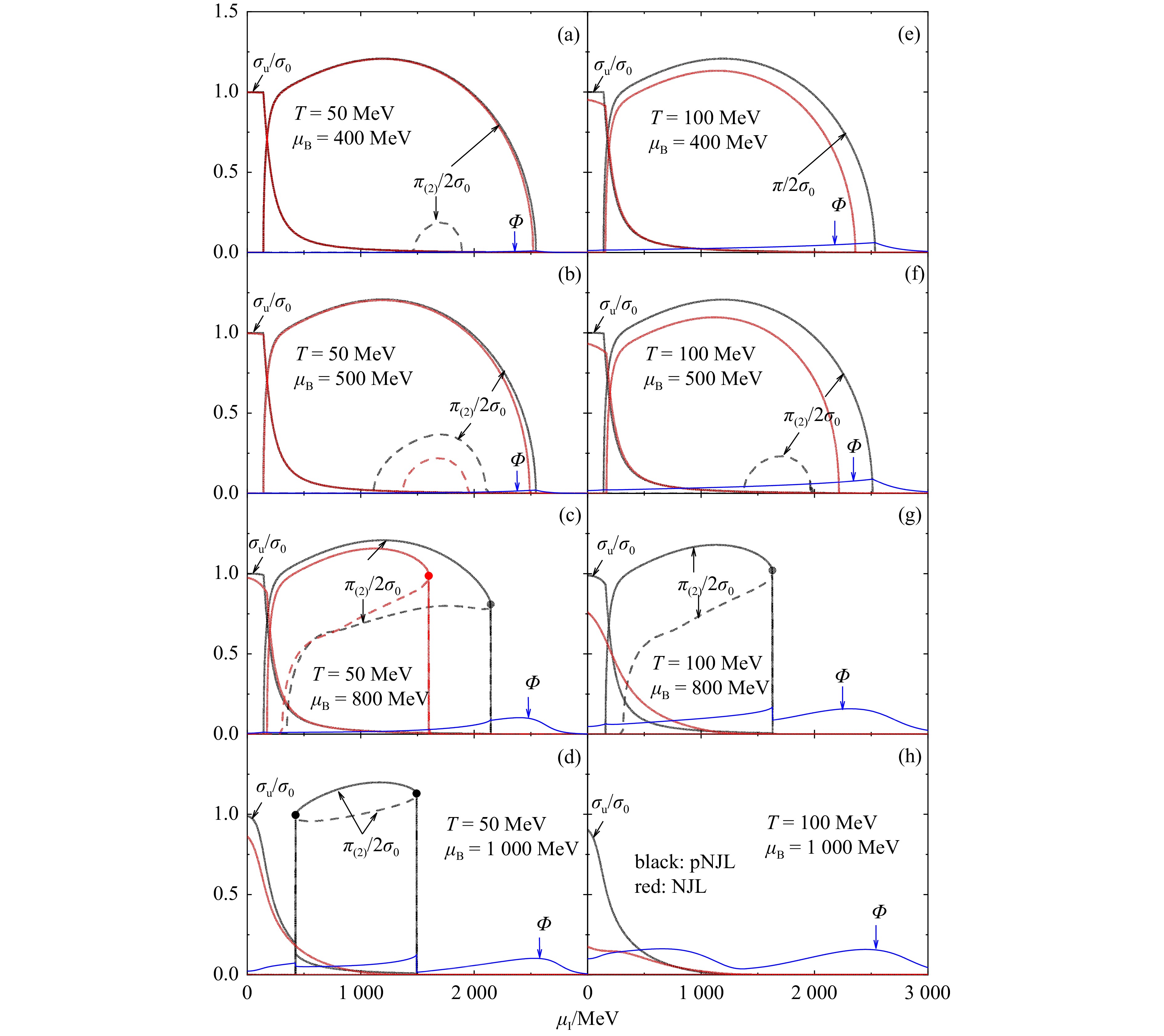
We compare the pion and chiral condensates in baryon-rich quark matter at $T = 50$ and 100 MeV as a function of the isospin chemical potential based on the NJL and pNJL model in Fig. 1. One sees that the pion condensate appears around $ \mu_\mathrm{I}^{} \sim m_\pi^{} $ and disappears at very large $ \mu_\mathrm{I}^{} $ or high temperatures. The appearance and disappearance of the pion condensate are second-order phase transitions at smaller $ \mu_\mathrm{B}^{} $. With the increasing $ \mu_\mathrm{B}^{} $, the disappearance of the pion condensate first becomes a first-order phase transition, and then the appearance of the pion condensate becomes a first-order one as well. At very large $ \mu_\mathrm{B}^{} $, there is no pion condensate. At intermediate $ \mu_\mathrm{B}^{} $, there exists a second nonzero solution $ \pi_2^{} $ (denoted as dashed lines), which corresponds to the local maximum of the thermodynamic potential and is called the Sarma phase^[64] as detailed in Ref. [31]. It is seen that the pion superfluid phase ($ \pi $) and the Sarma phase ($ \pi_2^{} $) exist in a broader region of chemical potentials and temperatures in the pNJL model than in the NJL model.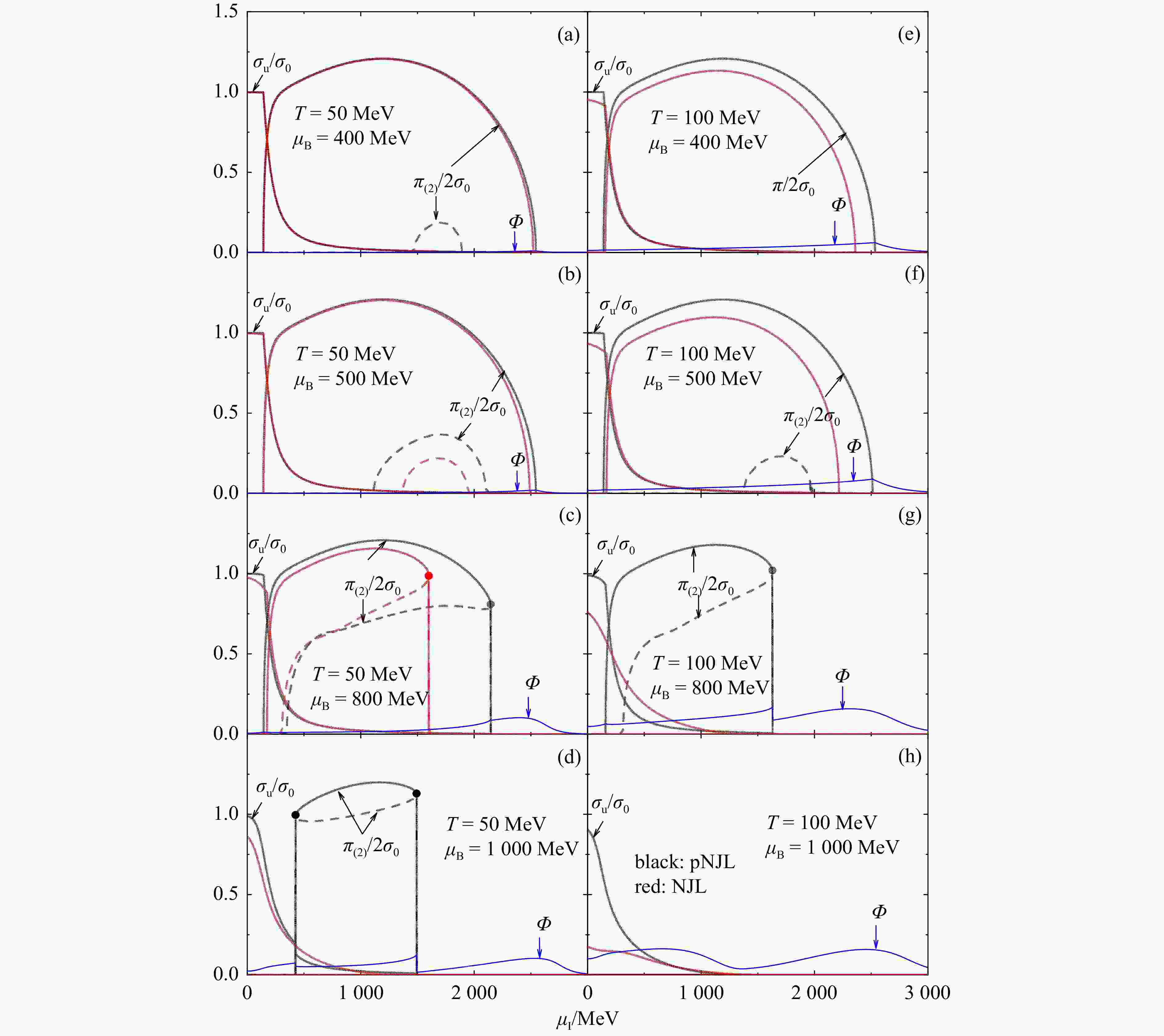

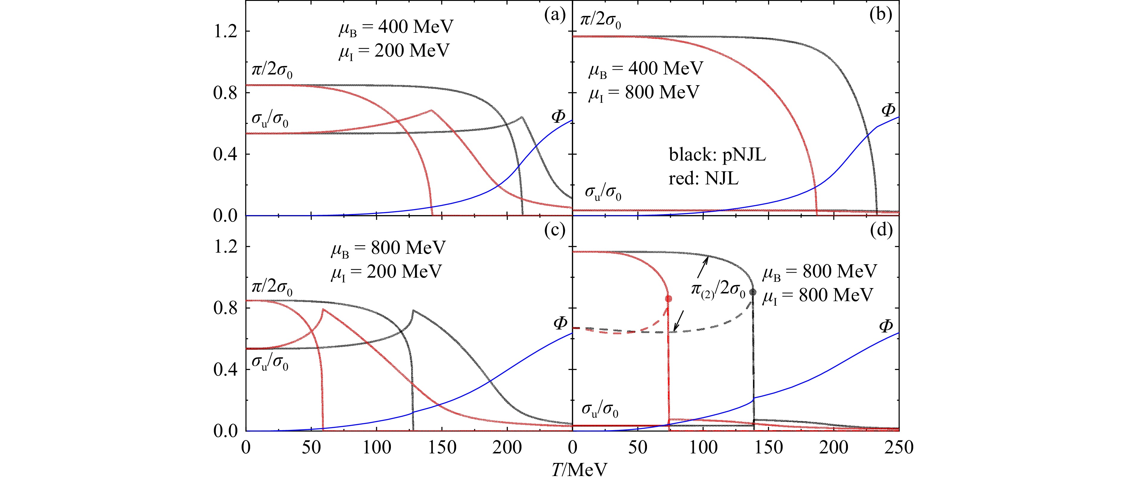
Figure 1.  Reduced pion condensate $\pi/2\sigma_0^{}$, Sarma phase solution $\pi_2^{}/2\sigma_0^{}$, and chiral condensate $\sigma_u^{}/\sigma_0^{}$ as well as the Polyakov loop $\varPhi$ as a function of the isospin chemical potential $\mu_\mathrm{I}^{}$ in hot [$T = 50$ (left) and $100$ (right) MeV] and baryon-rich [$\mu_\mathrm{B}^{} = 400$ (a),(e), 500 (b),(f), 800 (c),(g), and 1000 (d),(h) MeV] quark matter. Results are compared with those obtained from the NJL model. (color online)

Figure 2 displays the temperature dependence of the pion and chiral condensates at various baryon and isospin chemical potentials. One sees that the difference in the behavior of the pion condensate between the pNJL model and the NJL model is mainly at high temperatures. The temperatures for the disappearance of pion condensates $ \pi_{(2)}^{} $ in the pNJL model are much higher than those in the NJL model, which will manifest themselves in the results of the phase diagrams to be shown later. Again, the pion superfluid phase ($ \pi $) and the Sarma phase ($ \pi_2^{} $) exist in a broader region of temperatures in the pNJL model than in the NJL model.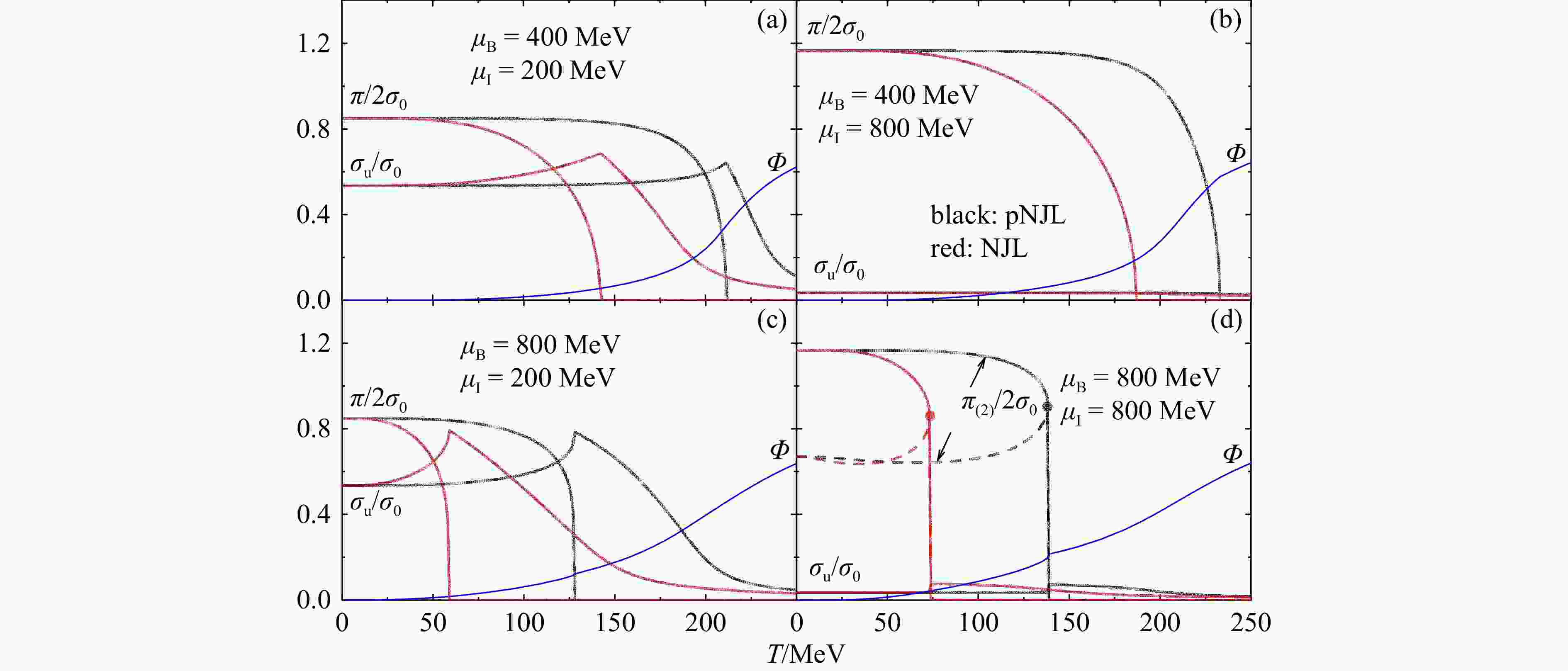

Figure 2.  Reduced pion condensate $\pi/2\sigma_0^{}$, Sarma phase solution $\pi_2^{}/2\sigma_0^{}$, and chiral condensate $\sigma_u^{}/\sigma_0^{}$ as well as the Polyakov loop $\varPhi$ as a function of the temperature $T$ in quark matter of different baryon chemical potentials $\mu_\mathrm{B}^{}$ and isospin chemical potentials $\mu_\mathrm{I}^{}$. Results are compared with those obtained from the NJL model. (color online)

Some common features in Figs. 1 and 2 need further discussions. According to the expressions of $ g $ functions in Ref. [31] and the gap equations [Eqs. (22)~(28)], both the chiral condensate and the net-quark densities depend on the gap parameter $ \varDelta $ or equivalently on the pion condensate $ \pi_{(2)}^{} $. Therefore, the sudden change of $ \pi_{(2)}^{} $, corresponding to either a first-order or a second-order phase transition of the whole quark matter system, leads to a sudden jump of the chiral condensates, the net-number densities as well as the Polyakov loop $ \varPhi $. For the behavior of the Polyakov loop $ \varPhi $, in principle one expects that it should increase with both the increasing chemical potential and temperature (see, e.g., Fig. 10 in Ref. [21]), while the non-monotonical dependence of $ \varPhi $ on $ \mu_\mathrm{I}^{} $ in Fig. 1 is due to the momentum cutoff in Eq. (21) when evaluating Eq. (31).

We now compare the three-dimensional ($ T $, $ \mu_\mathrm{B}^{} $, $ \mu_\mathrm{I}^{} $) QCD phase diagram based on the pNJL model with that from the NJL model, and mainly focus on the phase structure relevant to the pion condensate. The resulting phase diagram will be shown in the $ T-\mu_{\rm{B}}^{} $, $ T-\mu_{\rm{I}}^{} $, and $ \mu_{\rm{B}}^{}-\mu_{\rm{I}}^{} $ planes in Figs. 3, 4, and 5, respectively, where areas of the normal baryon-rich and isospin-asymmetric quark matter with $ \pi = 0 $ (Phases I), the pion superfluid phase with $\pi \ne 0$ (Phase II), and the phase with both nonzero solutions of $ \pi $ and $ \pi_2^{} $ (Phase III) as well as the corresponding phase boundaries will be presented. The transitions between Phase I and Phase III are always a first-order one indicated by the solid line, while the transitions between Phase I and Phase II as well as those between Phase II and Phase III are always a second-order one indicated by the dashed lines and dash-dotted lines, respectively. The CEP is generally the crossing point for the three phases.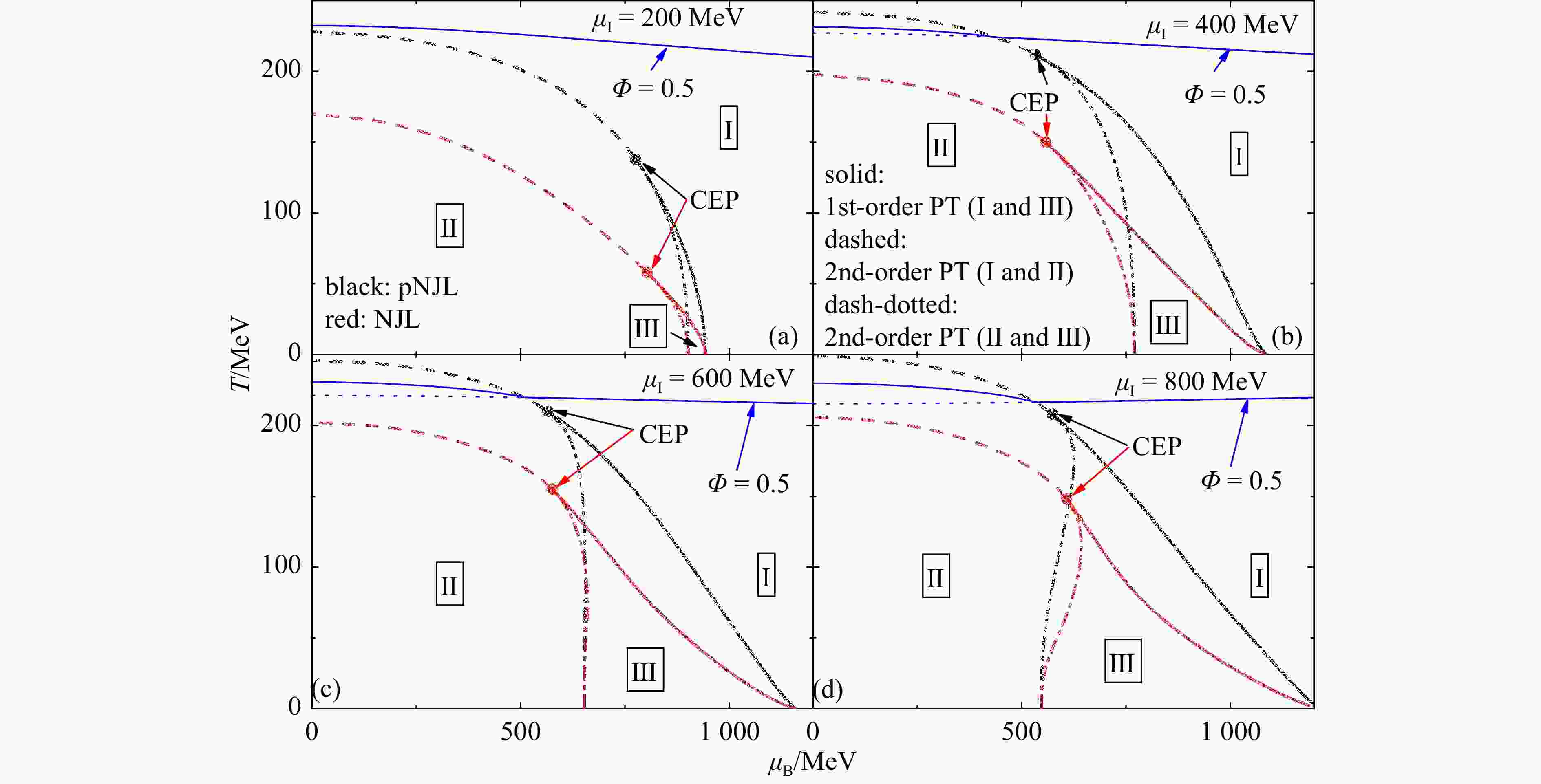

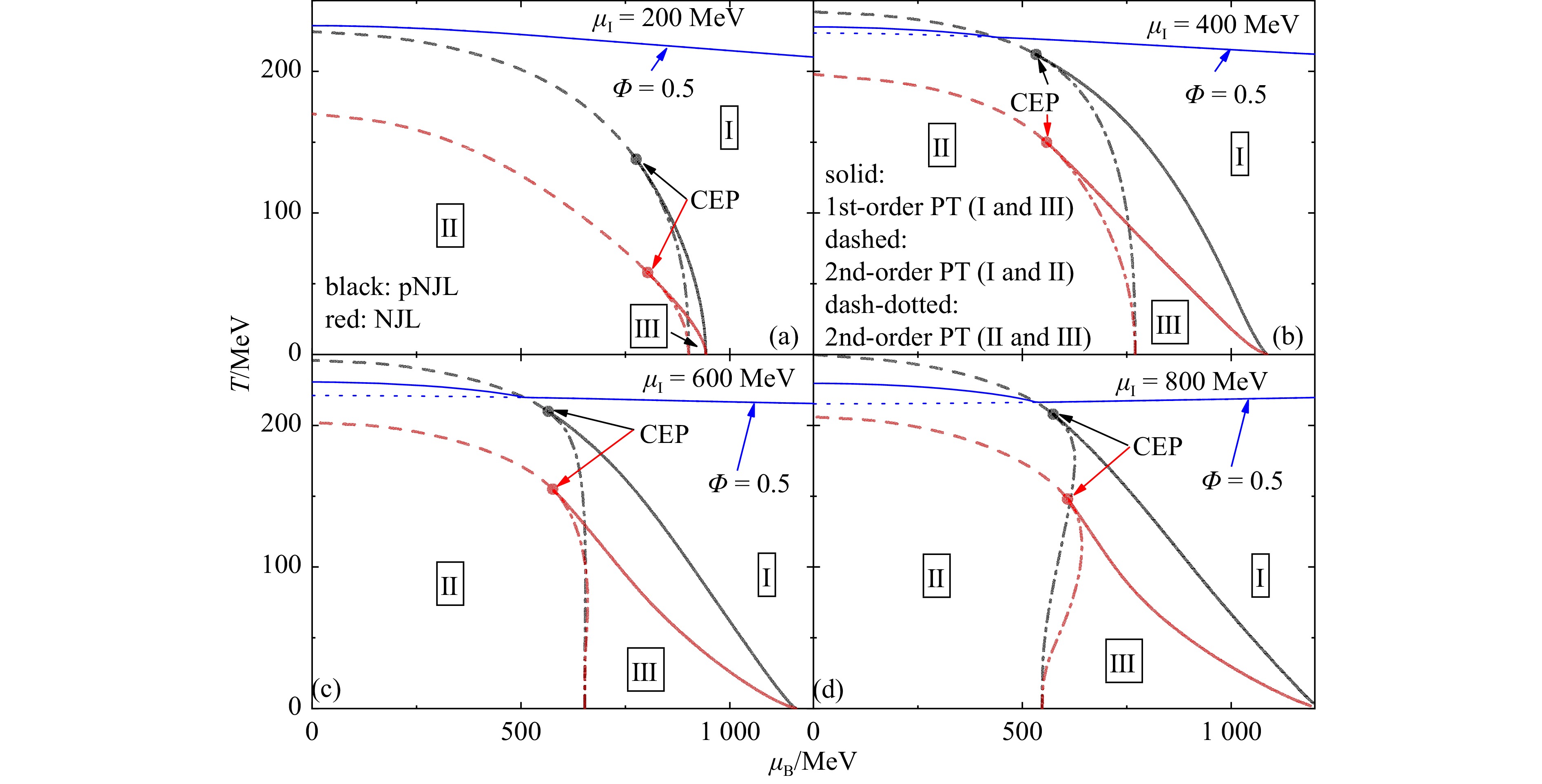
Figure 3.  Phase diagrams in the $T-\mu_\mathrm{B}^{}$ plane at different isospin chemical potentials $\mu_\mathrm{I}^{} = 200$ (a), 400 (b), 600 (c), and 800 (d) MeV in the pNJL model compared with those in NJL model. Solid lines represent the first-order phase transition (PT) between Phase I and Phase III, dashed lines represent the second-order phase transition between Phase I and Phase II, and dash-dotted lines represent the second-order phase transition between Phase II and Phase III. Blue solid (dotted) lines represent the deconfinement phase transition with (without) the pion condensate. (color online)

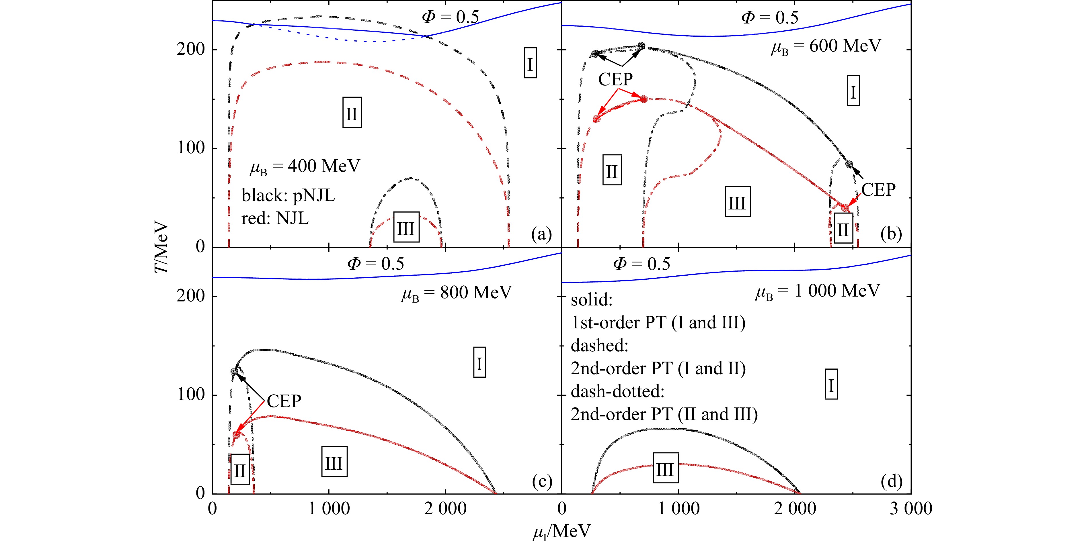
Figure 4.  Similar to Fig. 3 but in the $T-\mu_\mathrm{I}^{}$ plane at different baryon chemical potentials $\mu_\mathrm{B}^{} = 400$ (a), 600 (b), 800 (c), and 1 000 (d) MeV. (color online)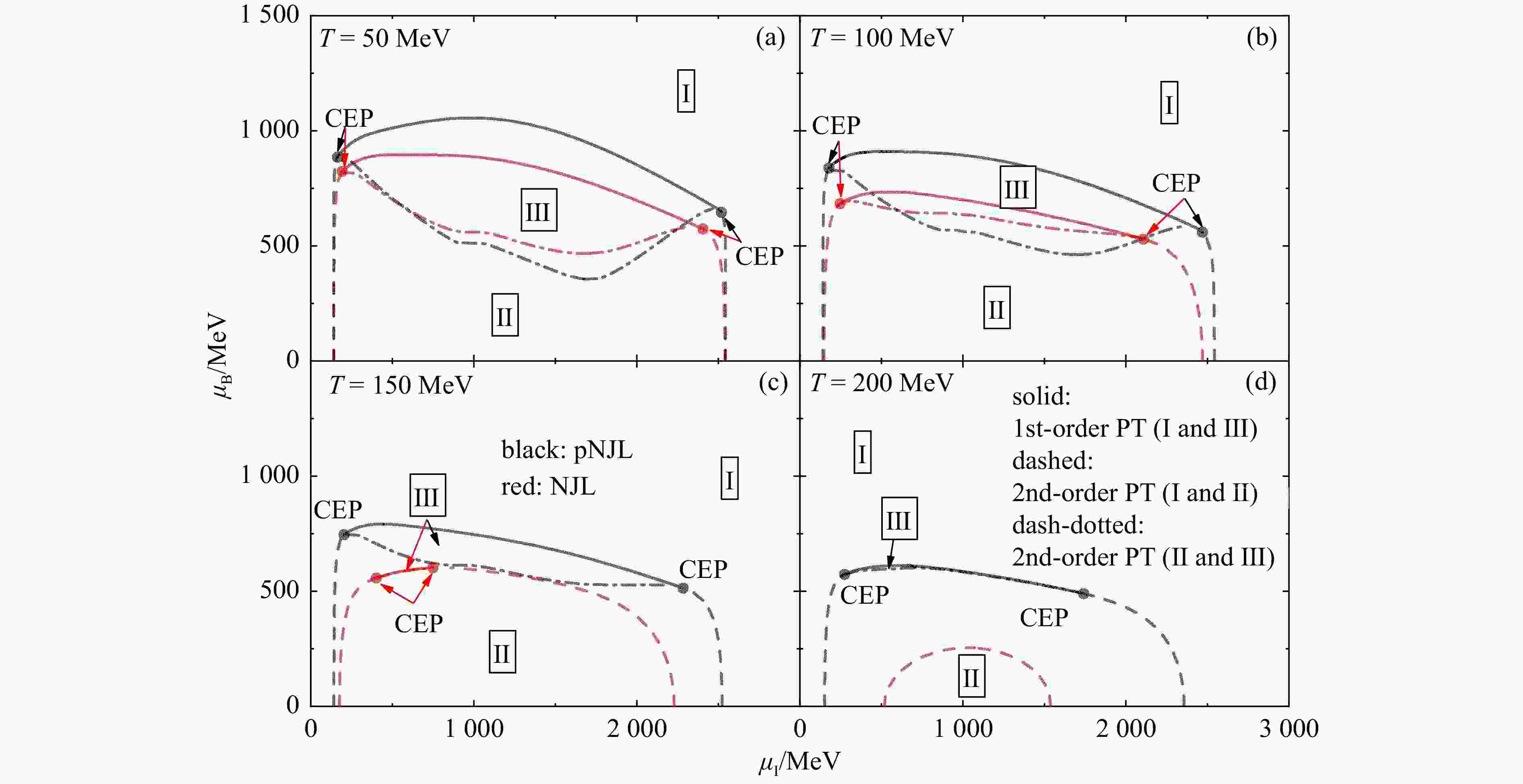

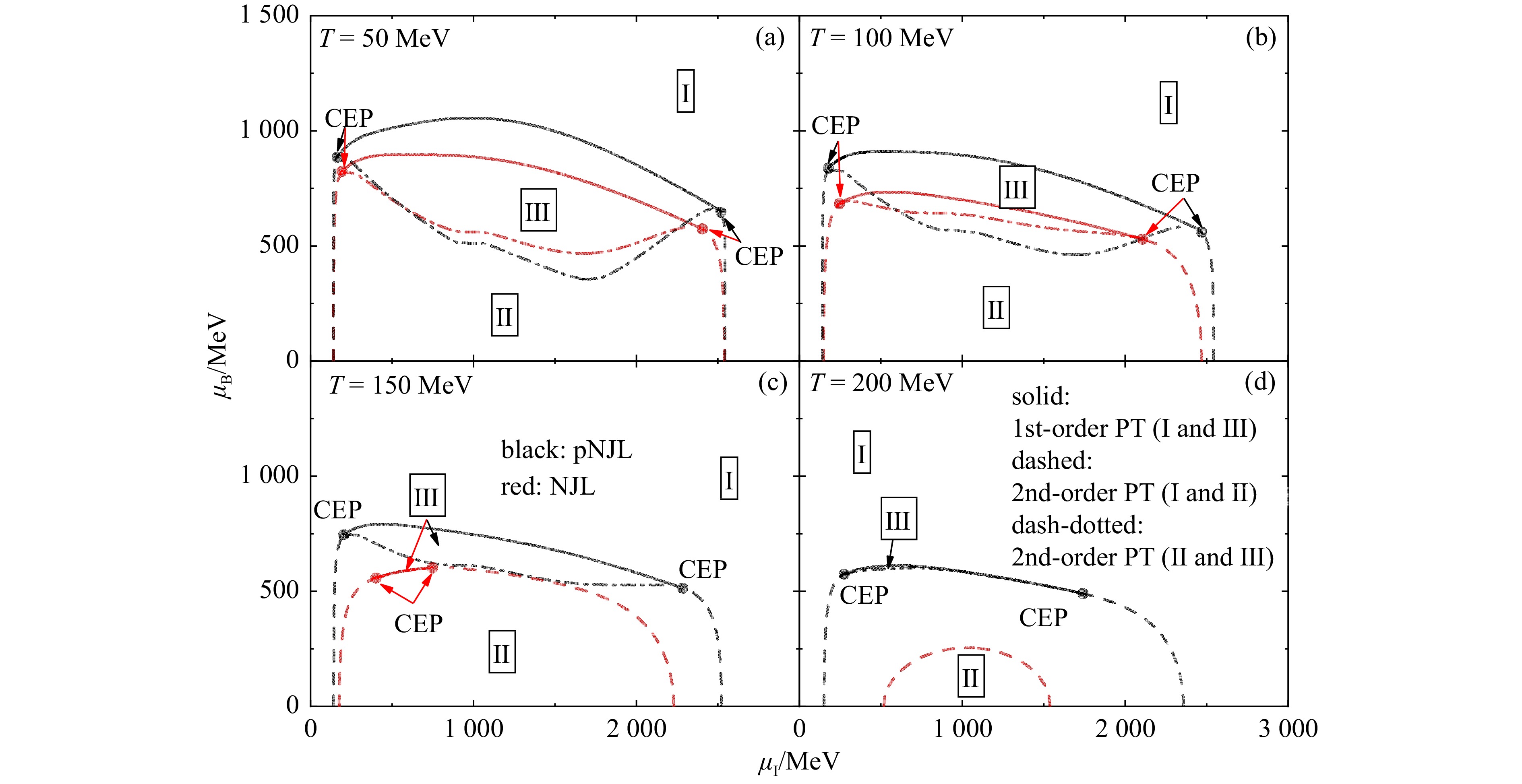
Figure 5.  Similar to Fig. 3 but in the $\mu_\mathrm{B}^{}-\mu_\mathrm{I}^{}$ plane at different temperatures $T = 50$ (a), 100 (b), 150 (c), and 200 (d) MeV. (color online)

Figure 3 displays the phase diagrams in the $ T-\mu_\mathrm{B}^{} $ plane at different isospin chemical potentials. For both NJL and pNJL models, Phase I generally exists at large $ T $ or large $ \mu_\mathrm{B}^{} $, while Phase II generally exists at small $ T $ and $ \mu_\mathrm{B}^{} $. The CEP connects the boundaries of the first-order phase transition and the second-order phase transitions, and it moves to a higher temperature when $ \mu_\mathrm{I}^{} $ changes from 200 to 400 MeV, while the increasing trend becomes saturated above $\mu_\mathrm{I}^{} = 400$ MeV. Compared to the NJL model, the pNJL model generally leads to larger areas of the pion superfluid phase and the Sarma phase, and a higher temperature of the CEP. Although the deconfinement phase transition in the pNJL model is always a smooth crossover, we plot an approximate deconfinement phase boundary obtained from $\varPhi = 0.5$ with blue solid lines, and at smaller $ \mu_\mathrm{B}^{} $ it moves slightly to lower temperatures if there is no pion condensate as shown by blue dotted lines.

Figure 4 displays the phase diagrams in the $ T-\mu_\mathrm{I}^{} $ plane at different baryon chemical potentials. For both NJL and pNJL models, the normal quark phase (Phase I) is obtained at very small or large isospin chemical potentials, or at high temperatures. It is seen that the area of the pion superfluid phase (Phase II) becomes smaller with the increasing baryon chemical potential. Second-order phase transitions are observed at small baryon chemical potentials, while first-order phase transitions occur at large baryon chemical potentials. Although not shown here, we find that Phase III with $\pi_2^{} \ne 0$ doesn't exist at $\mu_\mathrm{B}^{} = 0$, but it gradually appears inside Phase II at small baryon chemical potentials, and the area of Phase III generally increases with the increasing baryon chemical potential. Similar to that in the $ T-\mu_\mathrm{B}^{} $ plane, the pNJL model leads to larger areas of the pion superfluid and Sarma phases and higher temperatures of the CEPs, compared to the NJL model. The deconfinement phase transition occurs at high temperatures, and is affected by the pion condensate at smaller $ \mu_\mathrm{B}^{} $ and moderate $ \mu_\mathrm{I}^{} $.

Figure 5 displays the phase diagrams in the $ \mu_\mathrm{B}^{}-\mu_\mathrm{I}^{} $ plane at different temperatures. For both NJL and pNJL models, the normal quark phase (Phase I) exists at larger $ \mu_\mathrm{B}^{} $ and/or very small or large $ \mu_\mathrm{I}^{} $, and the pion superfluid phase (Phase II) is observed at smaller $ \mu_\mathrm{B}^{} $ and moderate $ \mu_\mathrm{I}^{} $, already seen in Figs. 3 and 4. The area of Phase II becomes smaller with the increasing temperature. Also, the first-order phase transition and Phase III gradually disappear with the increasing temperature. Similarly, the pNJL model leads to larger areas of the pion superfluid and Sarma phases and CEPs at larger baryon chemical potentials, compared to the NJL model.

To summarize, by introducing the gauge field and the Polyakov effective potential into the Lagrangian density of the extended three-flavor NJL model, we have studied the interplay among the chiral condensate, the pion condensate, and the Polyakov loop at finite temperatures, baryon chemical potentials, and isospin chemical potentials, and compared the three-dimensional QCD phase diagrams obtained from the NJL and pNJL models. While the two models give qualitatively similar QCD phase structures, we found that the pNJL model generally leads to larger areas of the pion superfluid phase and the Sarma phase, and the CEPs at higher temperatures. While the pion superfluid phase is stable, the Sarma phase corresponding to the local maximum of the thermodynamic potential is unstable against spatially inhomogeneous fluctuations, which can lead to the emergence of the Larkin-Ovchinnikov-Fudde-Ferrell phase^[65] or other spatially separated phases. The present study, which includes effectively the gluon dynamics, provides a more reliable prediction of the three-dimensional QCD phase diagram compared to our previous study.

As is well-known, NJL-type models are not normalizable and a momentum cutoff is generally needed to avoid divergence in the integral. While the results, especially at large chemical potentials, do depend the regularization, the Pauli-Villars regularization scheme^[66-67] could be a better choice compared to the sharp momentum cutoff, and can be investigated in future studies.

Acknowledgments We acknowledge helpful discussions with Zhen-Yan Lu. Jun Xu is supported by the Strategic Priority Research Program of the Chinese Academy of Sciences under Grant No. XDB34030000, the National Natural Science Foundation of China under Grant No. 12375125, and the Fundamental Research Funds for the Central Universities. Lu-Meng Liu and Guang-Xiong Peng are supported by the National Natural Science Foundation of China under Grant Nos. 11875052, 11575190, and 11135011.